MG-TSD; Multi-Granuality Time Series Diffusion Models with Guided Learning Process

MG-TSD: Multi-Granuality Time Series Diffusion Models with Guidedd Learning Process

Contents

1. Abstract
2. Introduction
3. Background
   1. DDPM
   2. TimeGrad
   3. Problem Formulation
4. Method
   1. MG-TSD Architecture
   2. Multi-Granularity Guided Diffusion
5. Expeirments

0. Abstract

TS forecasting with diffusion

\(\rightarrow\) remains an open question

\(\because\) Challenge of instability arising from their stochastic nature

Solution: propose MG-TSD (Multi-Granularity Time Series Diffusion)

• Leverage the inherent granularity levels within data

Intuition

• Forward process (sequentially corrupts the data)

  == Process of smoothing fine-grained data into coarse-grained representation

Proposal: Multi-granularity guidance diffusion loss function

• effectively utilize coarse-grained data across various granularity levels

1. Introduction

To stabilize the output of diffusion model in TS prediction….

\(\rightarrow\) Constrain the intermediate states during the sampling process

Previous solutions

• classifier guidance
• classifer-free guidance

\(\rightarrow\) Predicted posterior mean is shifted with the gradient of either explicit or implicit classifier

Limitations: require labels as the source of guidance while sampling

( unavailable during out-of-sample inference )

2. Background

(1) DDPM

\(L_n^{\text {simple }}=\mathbb{E}_{\boldsymbol{\epsilon}, \boldsymbol{x}_0}\left[ \mid \mid \boldsymbol{\epsilon}_n-\boldsymbol{\epsilon}_\theta\left(\sqrt{\bar{\alpha}_n} \boldsymbol{x}_0+\sqrt{1-\bar{\alpha}_n} \boldsymbol{\epsilon}, n\right) \mid \mid ^2\right]\).

(2) TimeGrad

\(\mathbb{E}_{\boldsymbol{\epsilon}, \boldsymbol{x}_{0, t}, n}\left[ \mid \mid \boldsymbol{\epsilon}-\boldsymbol{\epsilon}_\theta\left(\sqrt{\bar{\alpha}_n} \boldsymbol{x}_{0, t}+\sqrt{1-\bar{\alpha}_n} \boldsymbol{\epsilon}, n, \mathbf{h}_{t-1}\right) \mid \mid ^2\right]\).

• \(\mathbf{h}_t=\mathrm{RNN}_\psi\left(\boldsymbol{x}_t, \mathbf{h}_{t-1}\right)\).

(3) Problem Formulation

Notation

• Original observed data: \(\boldsymbol{X}^{(1)}=\left[\boldsymbol{x}_1^1, \ldots, \boldsymbol{x}_t^1, \ldots, \boldsymbol{x}_T^1\right]\), where \(\boldsymbol{x}_t \in \mathbb{R}^D\).

TS prediction task

• Model the conditional distribution of future timesteps time series \(\left[\boldsymbol{x}_{t_0}^1, \ldots, \boldsymbol{x}_T^1\right]\) given the fixed window of history context.
• \(q_{\mathcal{X}}\left(\boldsymbol{x}_{t_0: T}^1 \mid\left\{\boldsymbol{x}_{1: t_0-1}^1\right\}\right)=\prod_{t=t_0}^T q_{\mathcal{X}}\left(\boldsymbol{x}_t^1 \mid\left\{\boldsymbol{x}_{1: t-1}^1\right\}\right)\).

3. Method

• Section 3.1) MG-TSD model architecture
• Section 3.2) Novel guided diffusion process module

(1) MG-TSD Architecture

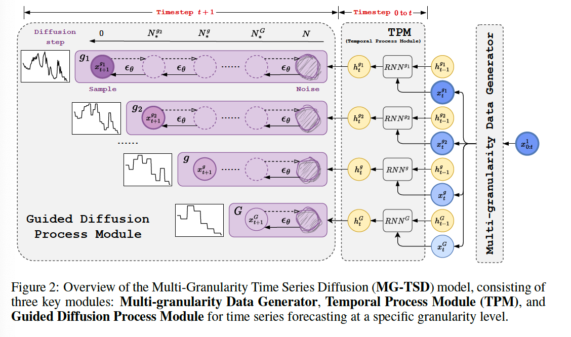
a) Multi-granularity Data Generator

• To generate multi-granularity data from observations

• By smoothing out the fine-grained data using historical sliding windows with different sizes

• Notation

  • \(f\) : smoothing (for example, average) function
  • \(s^g\) : sliding window size (for granularity level \(g\))
    • non-overlapping

  \(\rightarrow\) \(\boldsymbol{X}^{(g)}=f\left(\boldsymbol{X}^{(1)}, s^g\right)\).

• Obtained coarse-grained data for granularity \(g\) are replicated \(s^g\) times for alignment

b) Temporal Process Module

• To capture the temporal dynamics
• Utilize RNN on each granularity level \(g\) separately
  • Encoded hidden states : \(\mathbf{h}_t^g\).

c) Guided Diffusion Process Module

• To generate stable TS predictions at each timestep \(t\).
• Utilize multi-granularity data as given targets to guide the diffusion learning process.

(2) Multi-Granularity Guided Diffusion

• Section 3.2.1) Derivation of heuristic guidance loss for 2 granularity case
• Section 3.2.2) Generalizez loss to multi-granularity case

a) Coarse-Grained Guidance

Notation

• Finest-grained data \(\boldsymbol{x}_t^{g_1}\left(g_1=1\right)\) …. from \(\boldsymbol{X}^{\left(g_1\right)}\)

  & Coarse-grained data \(x_t^g\) ……………. from \(\boldsymbol{X}^{(g)}\)

• Approximate the distribution \(q\left(\boldsymbol{x}^{g_1}\right)\)
• Variance schedule : \(\left\{\beta_n^1=1-\alpha_n^1 \in(0,1)\right\}_{n=1}^N\).

Suppose \(x_0^{g_1} \sim q\left(x_0^{g_1}\right)\),

• Forward trajectory \(q\left(x_{0: N}^{g_1}\right)\)
• \(\theta\)-parameterized reverse trajectory \(p_\theta\left(x_{0: N}^{g_1}\right)\).

Proposal: guide the generation of samples by ensuring that the intermediate latent space retains the underlying time series structure

\(\rightarrow\) By introducing coarse-grained targets \(\boldsymbol{x}^g\) at intermediate diffusion step \(N_*^g \in[1, N-1]\).

Objective function \(\log p_\theta\left(\boldsymbol{x}^g\right)\)

• Evaluated at the marginal distributions at diffusion step \(N_*^g\),

  ( Need an appropriate choice of diffusion step \(N_*^g\), )

Marginal distribution of latent variable at denoising step \(N_*^g\)

• \(p_\theta\left(x_{N_*^g}\right)=\int p_\theta\left(x_{N_*^g: N}\right) \mathrm{d} x_{\left(N_*^g+1\right): N}=\int p\left(x_N\right) \prod_{N_*^g+1}^N p_\theta\left(x_{n-1} \mid x_n\right) \mathrm{d} x_{\left(N_*^g+1\right): N}\).
  • where \(\boldsymbol{x}_N \sim \mathcal{N}(\mathbf{0}, \boldsymbol{I}), p_\theta\left(\boldsymbol{x}_{n-1} \mid \boldsymbol{x}_n\right)=\mathcal{N}\left(\boldsymbol{x}_{n-1} ; \boldsymbol{\mu}_\theta\left(\boldsymbol{x}_n, n\right), \boldsymbol{\Sigma}_\theta\left(\boldsymbol{x}_n, n\right)\right)\).

To make the objective tractable … ELBO

• achieved by specifying a latent variable sequence of length \(N-N_*^g\)
• employ a diffusion process on \(\boldsymbol{x}^g\) with a total of \(N-N_*^g\) diffusion steps
  • defining a sequence of noisy samples \(x_{N_*^g+1}^g, \ldots, x_N^g\) as realizations of the latent variable sequence.
• Guidance objective:
  • \(\log p_\theta\left(\boldsymbol{x}^g\right)=\log \int p_\theta\left(\boldsymbol{x}_{N_*^g}^g, \boldsymbol{x}_{N_*^g+1}^g, \ldots, \boldsymbol{x}_N^g\right) \mathrm{d} \boldsymbol{x}_{\left(N_*^g+1\right): N^*}^g\).

Simplify the loss function!

• \(\mathbb{E}_{\epsilon, \boldsymbol{x}^g, n}\left[ \mid \mid \epsilon-\epsilon_\theta\left(\boldsymbol{x}_n^g, n\right) \mid \mid ^2\right]\).
  • \(\boldsymbol{x}_n^g=\left(\prod_{i=N_*^g}^n \alpha_i^1\right) x^g+\sqrt{1-\prod_{i=N_*^g}^n \alpha_i^1} \epsilon\) and \(\epsilon \sim \mathcal{N}(\mathbf{0}, \boldsymbol{I})\).
• If variance schedule : \(\left\{\alpha_n^1\right\}_{n=N^g}^N\),
  • Same as \(\log p_\theta\left(\boldsymbol{x}^g\right)=\log \int p_\theta\left(\boldsymbol{x}_{N_*^g}^g, \boldsymbol{x}_{N_*^g+1}^g, \ldots, \boldsymbol{x}_N^g\right) \mathrm{d} \boldsymbol{x}_{\left(N_*^g+1\right): N^*}^g\)

b) Multi-Granularity Guidance

Data of different granularities : \(\boldsymbol{X}^{(1)}, \boldsymbol{X}^{(2)}, \ldots, \boldsymbol{X}^{(G)}\).

• guide the learning process of the diffusion model at different steps

  ( = serve as constraints along the sampling trajectory )

Share ratio: shared percentage of variance schedule between

• (1) the \(g\) th granularity data, where \(g \in\{2, \ldots, G\}\)
• (2) the finest-grained data

\(\rightarrow\) Define it as \(r_g:=1-\left(N_*^g-1\right) / N\).

• ex) For the finest-grained data, \(N_*^1=1\) and \(r^1=1\).

Variance schedule for granularity \(g\)

\(\alpha_n^g\left(N_*^g\right)= \begin{cases}1 & \text { if } n=1, \ldots, N_*^g \\ \alpha_n^1 & \text { if } n=N_*^g+1, \ldots, N\end{cases}\).

and \(\left\{\beta_n^g\right\}_{n=1}^N=\left\{1-\alpha_n^g\right\}_{n=1}^N\).

• \(a_n^g\left(N_*^g\right)=\prod_{k=1}^n \alpha_k^g\),
• \(b_n^g\left(N_*^g\right)=1-\) \(a_n^g\left(N_*^g\right)\).

\(N_*^1<N_*^2 \ldots<N_*^g<\ldots<N_*^G\),

• which represents the diffusion index for starting sharing the variance schedule

Conditional inputs for the model to generate TS at corresponding granularity levels

Guidance loss function \(L^{(g)}(\theta)\)

• for \(g\) th-granularity \(\boldsymbol{x}_{n, t}^g\) at timestep \(t\) and diffusion step \(n\),

• \(L^{(g)}(\theta)=\mathbb{E}_{\boldsymbol{\epsilon}, \boldsymbol{x}_{0, t}^g, n} \mid \mid \left(\boldsymbol{\epsilon}-\boldsymbol{\epsilon}_\theta\left(\sqrt{a_n^g} \boldsymbol{x}_{0, t}^g+\sqrt{b_n^g} \boldsymbol{\epsilon}, n, \mathbf{h}_{t-1}^g\right) \mid \mid _2^2\right.\).

  • where \(\mathbf{h}_t^g=\operatorname{RNN}_\theta\left(\boldsymbol{x}_t^g, \mathbf{h}_{t-1}^g\right)\)

Total Guidance loss function

( with \(G-1\) granularity levels of data )

• \(L^{\text {guidance }}=\sum_{g=2}^G \omega^g L^{(g)}(\theta)\),
  • where \(\omega^g \in[0,1]\) is a hyper-parameter controlling the scale of guidance from granularity \(g\).

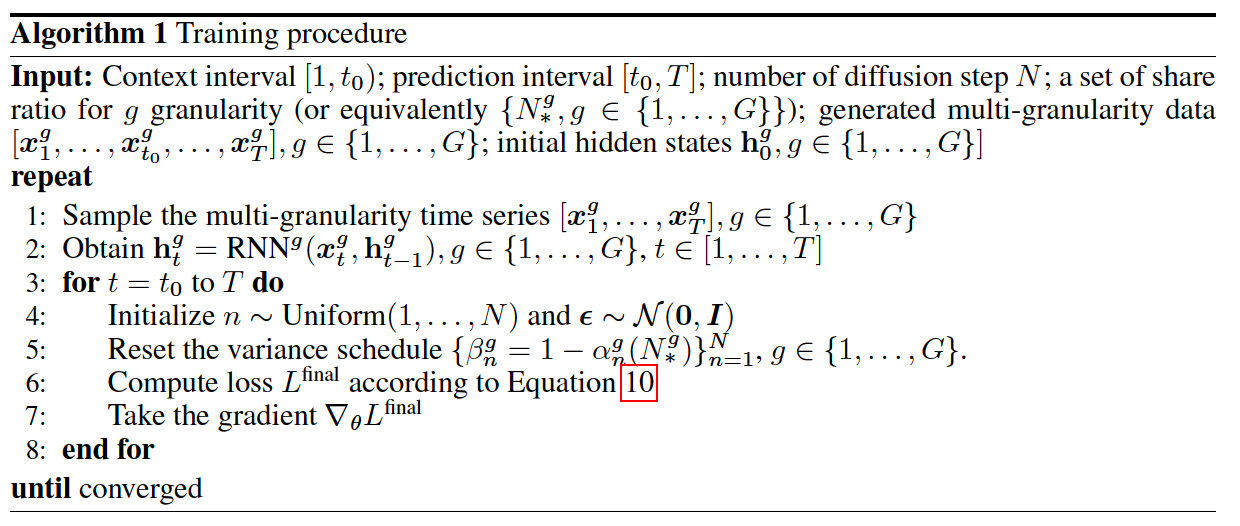
Training

\(L^{\text {final }}=\omega^1 L^{(1)}(\theta)+L^{\text {guidance }}(\theta)=\sum_{g=1}^G \omega^g \mathbb{E}_{\boldsymbol{\epsilon}, \boldsymbol{x}_{0, t}^g, n}\left[ \mid \mid \boldsymbol{\epsilon}-\boldsymbol{\epsilon}_\theta\left(\boldsymbol{x}_{n, t}^g, n, \mathbf{h}_{t-1}^g\right) \mid \mid ^2\right]\).

• denoising network parameters are shared across all granularities

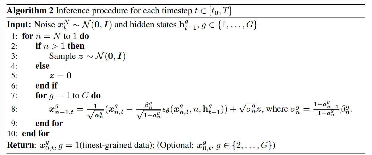
Inference

Goal: make predictions on the finest-grained data

Selection of share ratio

( heuristic approach )

\(N_*^g:=\arg \min _n \mathcal{D}\left(q\left(\boldsymbol{x}^g\right), p_\theta\left(\boldsymbol{x}_n^{g_1}\right)\right)\).

• i.e. \(\mathcal{D}\) : KL Divergence

4. Experiments

(1) Settings

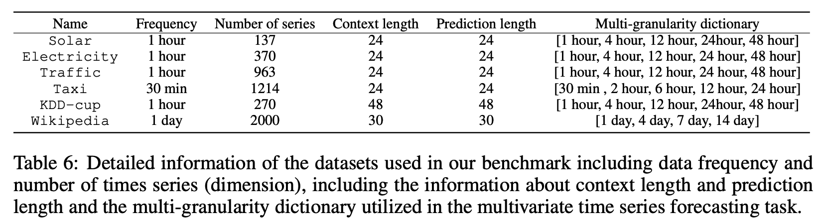
a) Datasets

6 Real-world datasets

• Characterized by a range of temporal dynamics
• Solar, Electricity, Traffic, Taxi, KDD-cup, Wikipedia
• Recorded at intervals of 30 minutes, 1 hour, or 1 day frequencies.

b) Evaluation Metrics

• CRPS (Continuous Ranked Probability Score)
• NMAE (Normalized Mean Absolute Error)
• NRMSE (Normalized Root Mean Squared Error)

c) Baselines

• Vec-LSTM-ind-scaling (Salinas et al., 2019)
• GP-scaling (Salinas et al., 2019)
• GP-Copula (Salinas et al., 2019)
• Transformer-MAF (Rasul et al., 2020)
• LSTM-MAF (Rasul et al., 2020)
• TimeGrad (Rasul et al., 2021)
• TACTiS (Drouin et al., 2022)
• MG-Input ensemble model
  • Baseline with multi-granularity inputs
  • Combines two TimeGrad models trained on one coarse-grained and finest-grained data respectively, and generates the final predictions by a weighted average of their outputs.

d) Implementation details

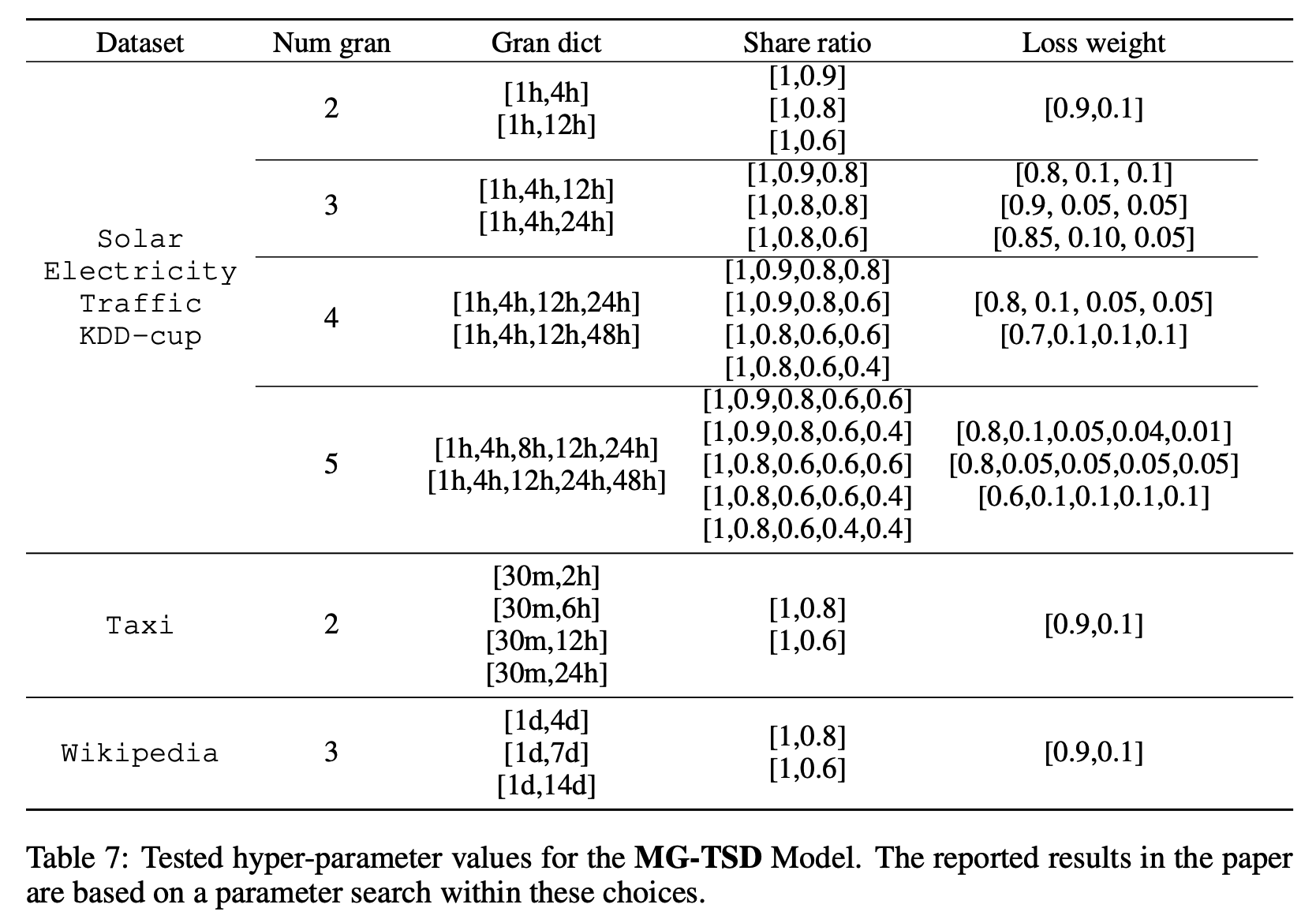
Hyperparameters

• 30 epochs using the Adam optimizer
• Fixed learning rate of \(10^{-5}\).
• Batch size to 128 for solar and 32 for other datasets
• Diffusion steps = 100

Additional hyperparameters

• share ratios
• granularity levels
• loss weights

(2) Results

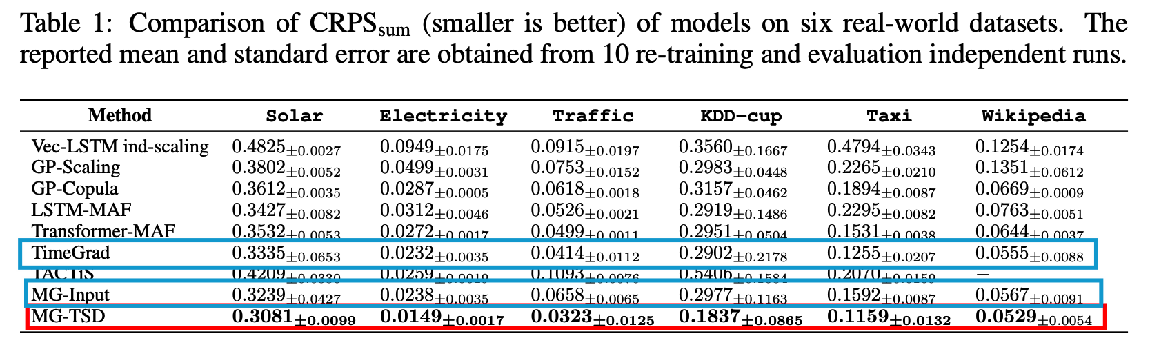
MG-Input model

• Marginal improvement on certain datasets when compared to the TimeGrad

  \(\rightarrow\) Integrating multi-granularity information may result in some information gain, but direct ensembling of coarse-grained outputs is inefficient!!

(3) Ablation Study

a) Share ratio of variance schedule

Various share ratios across different coarse granularities.

Two-granularity setting

• (1) Utilized to guide the learning process for the finest-grained data

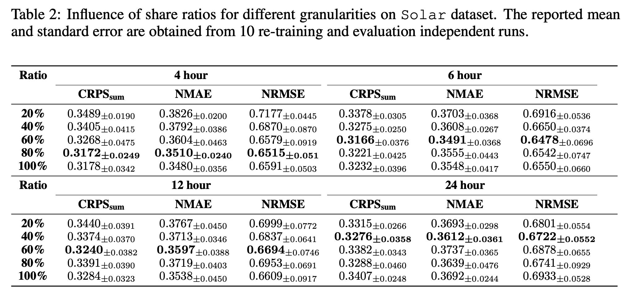
  • [Table 2]

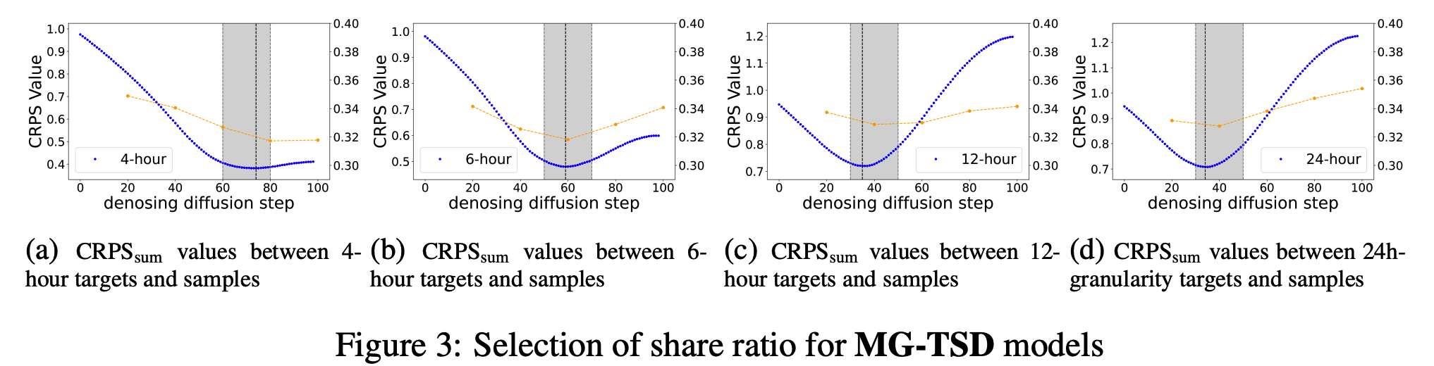
    • For each coarse granularity level, the CRPS \(_{\text {sum }}\) values initially decrease to their lowest values and then ascend again as the share ratio gets larger
    • For coarser granularities, the model performs better with a smaller share ratio.

    \(\rightarrow\) Suggests that the model achieves optimal performance when the share ratio is chosen at the step where the coarse-grained samples most closely resemble intermediate states

In practice, the selection of share ratio can follow the heuristic rule (Section 3.2.2)

• Strong correlation exists between the polyline of CRPS sum time and the share ratio selection curve

• As granularity transitions from fine to coarse \((4 h \rightarrow 6 h \rightarrow 12 h \rightarrow 24 h)\)…

  the diffusion steps at which the distribution most resembles the coarse-grained targets increase (approximately at steps \(20 \rightarrow 40 \rightarrow 60 \rightarrow 80)\).

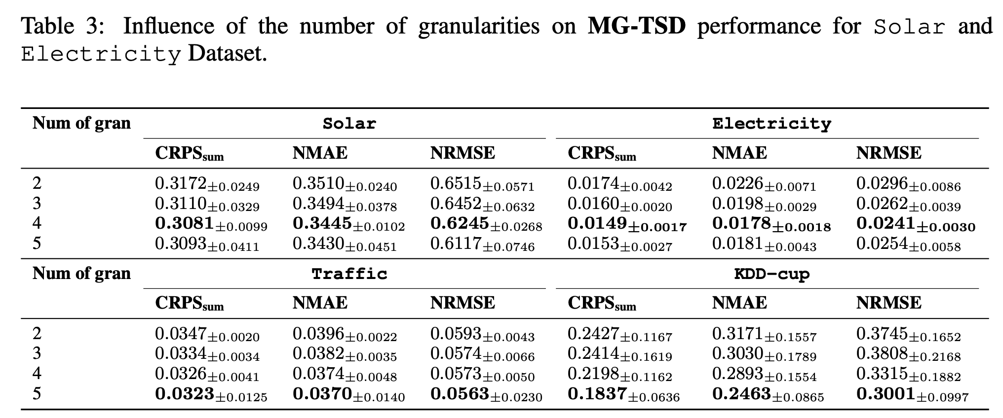
b) Number of granularity