(paper) Connecting the Dots ; MTS Forecasting with GNNs

Connecting the Dots ; MTS Forecasting with GNNs (2020, 147)

Contents

1. Abstract
2. Introduction
3. Problem Formulation
4. Framework of MTGNN
   1. Model Architecture
   2. Graph Learning Layer
   3. Graph Convolution Module
   4. Temporal Convolution Module
   5. Skipped Connection Layer & Output Module
   6. Proposed Learning Algorithm

Abstract

modeling MTS

• variables depend on each other!

  \(\rightarrow\) use GNN to capture relational dependencies!

propose a general GNN for MTS

• automatically extracts uni-direction relations among variables, through graph learning module

  ( external knowledge can be integrated )

• novel mix-hop propagation layer & dilated inception layer

  ( capture spatial & temporal dependencies )

• 3 components

  • (1) graph learning
  • (2) graph convolution
  • (3) temporal convolutions

  are jointly learned

1. Introduction

background of GNN’s success

• 1) permutation-invariance
• 2) local connectivity
• 3) compositionality

GNN for MTS : “spatial-temporal GNNs”

• input : MTS & external graph structures
• goal : predict future values/labels

challenges of those models

• 1) Unknown graph structure

  • rely heavily on pre-defined graph structure

    \(\rightarrow\) but in most cases, it doesn’t exists

• 2) Graph Learning & GNN Learning

  • most GNN focus only on “message passing” (GNN learning)

    ( ignore the fact that “graph structure isn’t optimal” )

  • so, how to learn those 2 simultaneously??

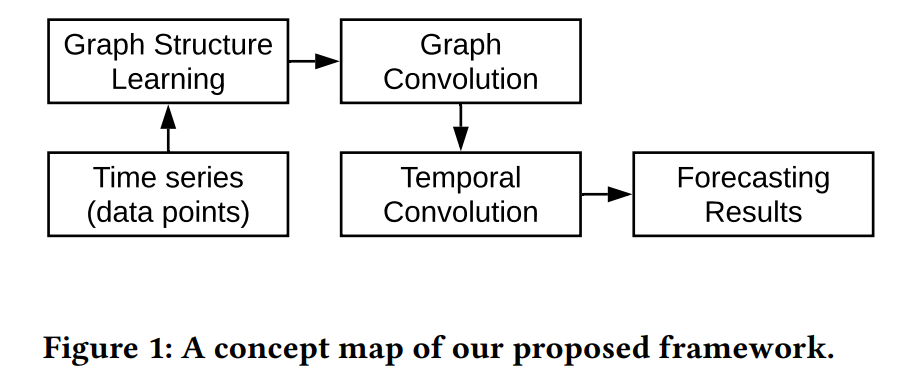
3 components ( all end-to-end )

• 1) graph learning layer
  • to overcome challenge (1)
• 2) graph convolution module
  • to capture spatial dependencies among variables
• 3) temporal convolution module
  • to capture temporal patterns, with modified 1d conv

Advantages : applicable to….

• 1) both small & large graphs,
• 2) both short & long TS,
• 3) with/without externally defined graph structures

2. Problem Formulation

Input = observed MTS : \(\mathrm{X}=\left\{\mathrm{z}_{t_{1}}, \mathrm{z}_{t_{2}}, \cdots, \mathrm{z}_{t_{P}}\right\}\)

• \(\mathbf{z}_{t} \in \mathbf{R}^{N}\) : multivariate variable of dimension \(N\) at time step \(t\)
  • \(z_{t}[i] \in R\) : value of the \(i^{t h}\) variable at time step \(t\)

Target :

• 1) \(Q\)-step-away value : \(\mathbf{Y}=\left\{\mathbf{z}_{t_{P+Q}}\right\}\)
• 2) sequence of future values : \(\mathbf{Y}=\left\{\mathbf{z}_{t_{P+1}}, \mathbf{z}_{t_{P+2}}, \cdots, \mathbf{z}_{t_{P+Q}}\right\}\)

Concatenated input signals

• \(\mathcal{X}=\left\{\mathrm{S}_{t_{1}}, \mathrm{~S}_{t_{2}}, \cdots, \mathrm{S}_{t_{P}}\right\}\).
  • \(\mathrm{S}_{t_{i}} \in \mathbf{R}^{N \times D}\), where \(D\) is feature dimension
    • first column : \(\mathrm{z}_{t_{i}}\)
    • other columns : auxiliary features

3. Framework of MTGNN

(1) Model Architecture

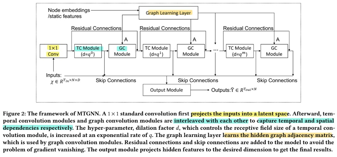
Components

• graph learning layer (1)
  • computes a graph adjacency matrix
  • used as an input to all graph convolution modules
• graph convolution modules (m)
  • capture spatial dependencies
• temporal convolution module (m)
  • capture temporal dependencies

ETC

• residual connections & skip connections

(2) Graph Learning Layer

goal : capture hidden relations among TS data

Similarity measure

• ex) dot product, Euclidean distance

[ Problem 1 ] high time & space complexity

• solution : sampling approach
  • only calculate pair-wise relationships among a subset of nodes

[ Problem 2 ] symmetric/bi-directional

• can not capture “cause” of the change

  ( should be uni-directional )

• solution :

  \(\begin{aligned} &\mathbf{M}_{1}=\tanh \left(\alpha \mathbf{E}_{1} \boldsymbol{\Theta}_{1}\right) \\ &\mathbf{M}_{2}=\tanh \left(\alpha \mathbf{E}_{2} \boldsymbol{\Theta}_{2}\right) \\ &\mathbf{A}=\operatorname{ReLU}\left(\tanh \left(\alpha\left(\mathbf{M}_{1} \mathbf{M}_{2}^{T}-\mathbf{M}_{2} \mathbf{M}_{1}^{T}\right)\right)\right) \\ &\text { for } i=1,2, \cdots, N \\ &\mathbf{i d x}=\operatorname{argtopk}(\mathbf{A}[i,:]) \\ &\mathbf{A}[i,-\mathbf{i d x}]=0, \end{aligned}\).

Incorporate external data

• if exists, can also set \(\mathbf{E}_1 = \mathbf{E}_2 = \mathbf{Z}\)

(3) Graph Convolution Module

Goal : handle spatial dependencies

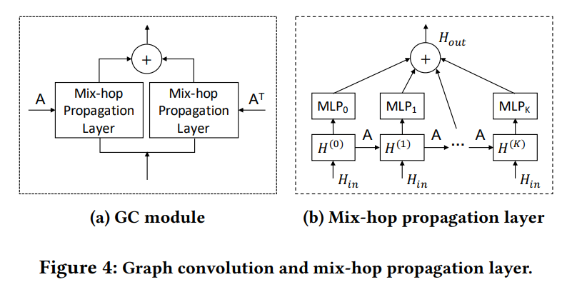
Consists of 2 mix-hop propogation layers

• consists of 2 steps
  • 1) information propagation step
    • \(\mathbf{H}^{(k)}=\beta \mathbf{H}_{i n}+(1-\beta) \tilde{\mathbf{A}} \mathbf{H}^{(k-1)}\).
  • 2) information selection step
    • \(\mathbf{H}_{o u t}=\sum_{i=0}^{K} \mathbf{H}^{(k)} \mathbf{W}^{(k)}\).
      • \(\mathbf{W}^{(k)}\) : act as “feature selector”
  • \(\mathbf{H}^{(0)}=\mathbf{H}_{i n}, \tilde{\mathbf{A}}=\) \(\tilde{\mathbf{D}}^{-1}(\mathbf{A}+\mathbf{I})\), and \(\tilde{\mathbf{D}}_{i i}=1+\sum_{j} \mathbf{A}_{i j} .\)

Concatenate information from different hops

(4) Temporal Convolution Module

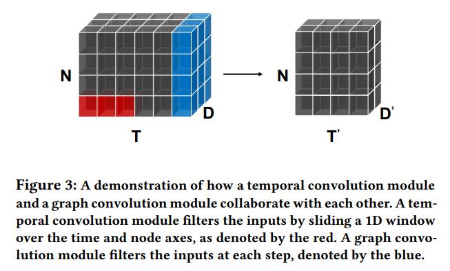
set of dilated 1d conv filters

consists of 2 layers

• 1) with tangent hyperbolic activation function
• 2) with sigmoid activation function

Dilated Inception Layer

able to both discover “temporal patterns” with various ranges

& handle “very long sequences”

\(\rightarrow\) propose a dilated inception layer

( use filters with multiple sizes & apply dilated convolution )

Details

• 1) consist of 4 filter sizes \(\rightarrow\) combination
• 2) dilated convolution, for larger receptive fields

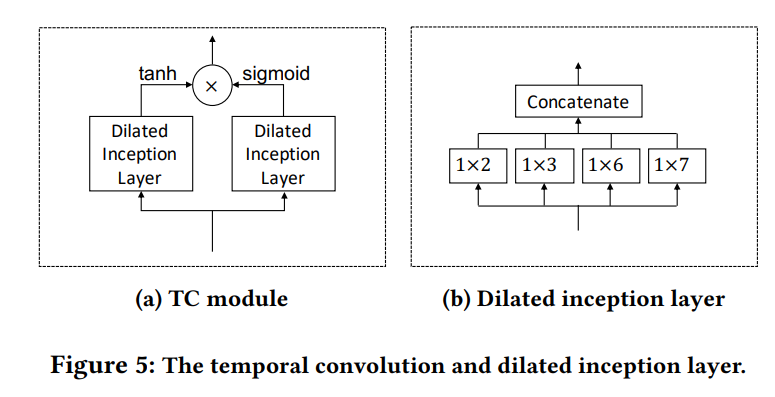
Combine inception & dilation

\(\mathbf{z}=\operatorname{concat}\left(\mathbf{z} \star \mathbf{f}_{1 \times 2}, \mathbf{z} \star \mathbf{f}_{1 \times 3}, \mathbf{z} \star \mathbf{f}_{1 \times 6}, \mathbf{z} \star \mathbf{f}_{1 \times 7}\right)\).

• where \(\mathbf{z} \star \mathbf{f}_{1 \times k}(t)=\sum_{s=0}^{k-1} \mathbf{f}_{1 \times k}(s) \mathbf{z}(t-d \times s)\)

(5) Skipped Connection Layer & Output Module

Skipped Connection

• to prevent gradient vanishing

Output module

• predict certain future step : output dim = 1
• predict \(Q\) future step : output dim = \(Q\)

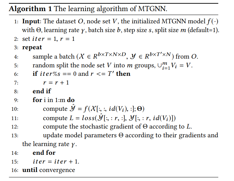
(6) Proposed Learning Algorithm