(paper) SAITS ; Self-Attention-based Imputation for TS

SAITS : Self-Attention-based Imputation for TS (2022)

Contents

1. Abstract

2. Related Work
3. Methodology
   1. Joint-Optimization Training Approach
   2. SAITS
      1. DMSA ( Diagonally Masked Self-Attention )
      2. Positional Encoding & Feed-forward Network
      3. First DMSA Block
      4. Second DMSA Block
      5. Weighted Combination Block
      6. Loss Functions

0. Abstract

SAITS

• self-attention
• for missing value imputation
• in MTS

Details

• joint optimization approaches
• learns missing values froma weighted combination of 2 DMSA blocks
  • DMSA = Diagonally-Masked Self-Attention block
• captures both …
  • “temporal dependencies”
  • “feature correlations between time steps”

1. Related Work

4 categories of TS imputation

(1) RNN-based

GRU-D

• GRU variant
• time decay on the last observation

M-RNN & BRITS

• impute missing values according to hidden states from bi-RNN
• difference
  • M-RNN : treats missing values as constants
  • BRITS : takes correlations among features

(2) GAN-based

• also RNN-based ( + GAN framework )

• G & Dare both based on GRUI

• since it is RNN-based…
  • time-consuming & memory constraints & long-term dependency problem

(3) VAE-based

• GAN & VAE-based : difficult to train

(4) Self-attention based

CDSA

• cross-dimensional self-attention, from 3 dimensions
  • time / location / measurement
• impute missing values in geo-tagged data
• (problem) specifically designfed for spatiotemporal data

DeepMVI

• missing value imputation in multidimensional TS data

• (problem) not open-source

NRTIS

• TS imputation approach treating time series as a set of (time, data) tuples
• (problem) consists of 2 nested loops …..

2. Methodology

made up of 2 parts

• (1) joint-optimization of “imputation & reconstruction”
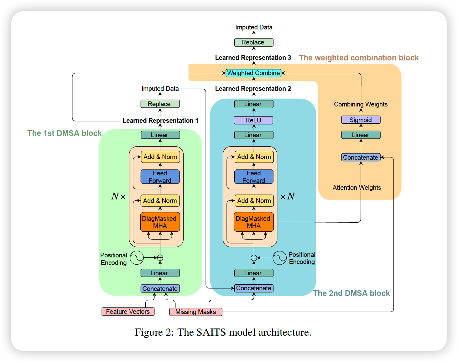
• (2) SAITS model ( =weighted combination of 2 DMSA blocks )

(1) Joint-Optimization Training Approach

Notation

• MTS : \(X=\left\{x_{1}, x_{2}, \ldots, x_{t}, \ldots, x_{T}\right\} \in \mathbb{R}^{T \times D}\).
  • \(t\)-th observation : \(x_{t}=\left\{x_{t}^{1}, x_{t}^{2}, \ldots, x_{t}^{d}, \ldots, x_{t}^{D}\right\}\)
• Missing mask vector : \(M \in \mathbb{R}^{T \times D}\)
  • \(M_{t}^{d}= \begin{cases}1 & \text { if } X_{t}^{d} \text { is observed } \\ 0 & \text { if } X_{t}^{d} \text { is missing }\end{cases}\).

2 learning tasks

• (1) MIT ( = Masked Imputation Task )
• (2) ORT ( = Observed Reconstruction Task )

\(\rightarrow\) two loss functions are added

Task 1 : MIT

Details :

• ARTIFICIALLY masked value ( predict this missing values )
• mask at random
• calculate imputation loss ( use MAE )

Notation

• \(\hat{X}\) : actual input feature vector
• \(\hat{M}\) : corresponding missing mask vector
• REAL vs FAKE missing : \(I\)

Mask vectors

\(\hat{M}_{t}^{d}=\left\{\begin{array}{ll} 1 & \text { if } \hat{X}_{t}^{d} \text { is observed } \\ 0 & \text { if } \hat{X}_{t}^{d} \text { is missing } \end{array}, \quad I_{t}^{d}= \begin{cases}1 & \text { if } \hat{X}_{t}^{d} \text { is artificially masked } \\ 0 & \text { otherwise }\end{cases}\right.\).

MLM vs MIT

• inspired by MLM
• difference
  • MLM : predicts missing tokens ( time steps )
  • MIT : predict missing values in time steps
• disadvantages of MLM : “discrepancy”
  • masking symbols used during pretraining are absent from real data in fine tuning
  • no such discrepancy in MIT!

Task 2 : ORT

• reconstruction task ( on the observed values )
• use MAE

Sumamry

• MIT : force the model to predict missing values as accurately as possible
• ORT : ensure that the model converge to the distn of observed data

(2) SAITS

composed of 2 DMSA blocks & weighted combination

a) DMSA ( Diagonally Masked Self-Attention )

( before )

• \[\text { SelfAttention }(Q, K, V)=\operatorname{Softmax}\left(\frac{Q K^{\top}}{\sqrt{d_{k}}}\right) V\]

( diagonal mask )

• \([\operatorname{DiagMask}(x)](i, j)= \begin{cases}-\infty & i=j \\ x(i, j) & i \neq j\end{cases}\).

( after )

• \(\operatorname{DiagMaskedSelfAttention}(Q, K, V) =\operatorname{Softmax}\left(\operatorname{DiagMask}\left(\frac{Q K^{\top}}{\sqrt{d_{k}}}\right)\right) V =A V\).

cannot see themselves

\(\rightarrow\) only on the input values from other \((T-1)\) time steps

\(\rightarrow\) able to capture temporal dependencies & feature correlations

b) Positional Encoding & Feed-forward Network

• skip

c) First DMSA Block

• skip

d) Second DMSA Block

• skip

e) Weighted Combination Block

\(\begin{gathered} \hat{A}=\frac{1}{h} \sum_{i}^{h} A_{i} \\ \eta=\operatorname{Sigmoid}\left(\operatorname{Concat}(\hat{A}, \hat{M}) W_{\eta}+b_{\eta}\right) \\ \tilde{X}_{3}=(1-\eta) \odot \tilde{X}_{1}+\eta \odot \tilde{X}_{2} \\ \hat{X}_{c}=\hat{M} \odot \hat{X}+(1-\hat{M}) \odot \tilde{X}_{3} \end{gathered}\).

• dynamically weiht \(\tilde{X_1}\) & \(\tilde{X_2}\)

f) Loss Functions

\(\begin{aligned} \ell_{\mathrm{MAE}}(\text { estimation, target, mask }) &=\frac{\sum_{d}^{D} \sum_{t}^{T} \mid(\text { estimation }-\text { target }) \odot \text { mask }\left. \mid _{t} ^{d}}{\sum_{d}^{D} \sum_{t}^{T} \text { mask }_{t}^{d}} \\ \mathcal{L}_{\mathrm{ORT}}=\frac{1}{3}\left(\ell_{\mathrm{MAE}}\left(\tilde{X}_{1}, \hat{X}, \hat{M}\right)\right.&\left.+\ell_{\mathrm{MAE}}\left(\tilde{X}_{2}, \hat{X}, \hat{M}\right)+\ell_{\mathrm{MAE}}\left(\tilde{X}_{3}, \hat{X}, \hat{M}\right)\right) \\ \mathcal{L}_{\mathrm{MIT}} &=\ell_{\mathrm{MAE}}\left(\hat{X}_{c}, X, I\right) \\ \mathcal{L} &=\mathcal{L}_{\mathrm{ORT}}+\mathcal{L}_{\mathrm{MIT}} \end{aligned}\).