(paper) Mixing Up Contrastive Learning ; Self-Supervised Representation Learning for TS

Mixing Up Contrastive Learning : Self-Supervised Representation Learning for TS (2022)

Contents

1. Abstract
2. Introduction
3. Mixup Contrastive Learning
   1. Novel Contrastive Loss

0. Abstract

lack of labeled data

\(\rightarrow\) need for UNsupervised representation framework

propose an UNSUPERVISED CONTRASTIVE LEARNING framework,

• motivated from the perspective of label smoothing

• use a novel contrastive loss,

  • That exploits a data augmentation scheme

    ( = new samples : generated by mixing 2 data samples )

• task : predict the mixing component

  ( = which is utilized as soft targets in the loss function )

1. Introduction

Contrastive Learning

• self-supervised reprsentation learning

• key : discriminate between different view of the sample

  • different view = created via data augmentation

    ( exploit prior information about the structure in the data )

  • data augmentation :

    • usually done by injecting noise

Data Augmentation for TS

• more challengfing, due to…
• (1) heterogeneous nature of TS data
• (2) lack of generally applicable augmentations

Mixup

• recent data augmentation scheme

• creates an augmented sample, via…

  \(\rightarrow\) convex combination of 2 data poionts & mixing component

Proposed framework

• Task : predict the strength of the mixing component,
  • based on the “2 data points & augmented samples”
• motivated by LABEL SMOOTHING
  • concept of adding noise to the labels
  • soft target : between 0~1

2. Mixup Contrastive Learning

explain based on UTS (Univariate Time Series)

• \(x=\{x(t) \in \mathbb{R} \mid t=1,2, \cdots, T\}\).

Common approach in Contrastive learning

• ENCODER : \(x \rightarrow z\)
  • encoder is trained by passing different augmentations of the SAME sample
• goal of contrastive learning
  • embed similar samples in close proximity by exploiting the INVARIANCES in the data
• after training, discared except ENCODER

Data Augmentation

• create new samples via convex combinations of training examples ( = Mixup )
• 2 time series ( \(x_i\) & \(x_j\) ) drawn randomly from data
• \(\tilde{x} = \lambda x_i + (1-\lambda) x_j\).
  • \(\lambda \in [0,1]\) : mixing parameters
    • \(\lambda \sim \text{Beta}(\alpha, \alpha)\) & \(\alpha \in (0, \infty)\)

\(\rightarrow\) task : predicting hard 0 & 1 targets to soft targets \(\lambda\) & \(1-\lambda\)

\(\rightarrow\) lead to increased performance & less overconfidence

(1) Novel Contrastive Loss

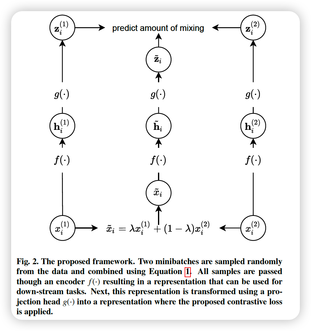
At each training iteration….

• (step 1) new \(\lambda\) is drawn ( from Beta distn )
• (step 2) draw 2 minibatches, of size \(N\)
  • (2-1) \(\left\{x_{1}^{(1)}, \cdots, x_{N}^{(1)}\right\}\)
  • (2-2) \(\left\{x_{1}^{(2)}, \cdots, x_{N}^{(2)}\right\}\)

• (step 3) create a new minibatch of AUGMENTED samples

  • \(\left\{\tilde{x}_{1}, \cdots, \tilde{x}_{N}\right\}\).

• (step 4) pass 3 minibatches to ENCODER \(f(\cdot)\)

  • (1) \(\left\{\mathbf{h}_{1}^{(1)}, \cdots, \mathbf{h}_{N}^{(1)}\right\}\)
  • (2) \(\left\{\mathbf{h}_{1}^{(2)}, \cdots, \mathbf{h}_{N}^{(2)}\right\}\)
  • (3) \(\left\{\tilde{\mathbf{h}}_{1}, \cdots, \tilde{\mathbf{h}}_{N}\right\}\)

  ( those three can be used for downstream tasks )

• (step 5) transform 3 mini batches into task-dependent representation

  • (1) \(\left\{\mathbf{z}_{1}^{(1)}, \cdots, \mathbf{z}_{N}^{(1)}\right\}\)
  • (2) \(\left\{\mathbf{z}_{1}^{(2)}, \cdots, \mathbf{z}_{N}^{(2)}\right\}\)
  • (3) \(\left\{\tilde{\mathbf{z}}_{1}, \cdots, \tilde{\mathbf{z}}_{N}\right\}\)

Proposed Contrastive loss for a single instance :

\(l_{i}=-\lambda \log \frac{\exp \left(\frac{D_{C}\left(\tilde{\mathbf{z}}_{i}, \mathbf{z}_{i}^{(1)}\right)}{\tau}\right)}{\sum_{k=1}^{N}\left(\exp \left(\frac{D_{C}\left(\tilde{\mathbf{z}}_{i}, \mathbf{z}_{k}^{(1)}\right)}{\tau}\right)+\exp \left(\frac{D_{C}\left(\tilde{\mathbf{z}}_{i}, \mathbf{z}_{k}^{(2)}\right)}{\tau}\right)\right)}\) \(-(1-\lambda) \log \frac{\exp \left(\frac{D_{C}\left(\tilde{\mathbf{z}}_{i}, \mathbf{z}_{i}^{(2)}\right)}{\tau}\right)}{\sum_{k=1}^{N}\left(\exp \left(\frac{D_{C}\left(\tilde{\mathbf{z}}_{i}, \mathbf{z}_{k}^{(1)}\right)}{\tau}\right)+\exp \left(\frac{D_{C}\left(\tilde{\mathbf{z}}_{i}, \mathbf{z}_{k}^{(2)}\right)}{\tau}\right)\right)}\),

• where \(D_{C}(\cdot)\) denotes the cosine similarity and \(\tau\) denotes a temperature parameter