
Univariate 3. 적분 선형확률 과정 ( Integrated Linear Process )
세부 알고리즘:
- ARIMA(Auto-Regressive Integrated Moving Average)
- SARIMA(Seasonal ARIMA)
6. ARIMA(Auto-Regressive Integrated Moving Average)
\[ARIMA(p,d,q)\]- 1) 1 이상의 차분이 적용된 \(\Delta^d Y_t = (1-L)^d Y_{t}\)가
- 2) 알고리즘의 차수(\(p,q\))가 유한한 \(AR(p)\)와 \(MA(q)\)의 Linear Combination
비정상성을 가진 time series \(Y_t\)를 차분하여 생성된 \(\Delta Y_t = Y_t - Y_{t-1} = (1-L) Y_{t}\)
- 1) 정상성을 따르고
- 2) ARMA 모형을 따르면
\(Y_t\)를 ARIMA 모형이라 한다
보다 general 하게, \(d\) 번 차분 한 경우 :
- 적분차수(Order of Integrarion)가 \(d\)인 ARIMA(p,d,q)
- example)
- \(p=0\): ARIMA(0,d,q) = IMA(d,q)
- \(q=0\): ARIMA(p,d,0) = ARI(p,d)
파라미터 소개
| Parameters | Description |
|---|---|
| \(p\) | order of the autoregressive part |
| \(d\) | degree of differencing involved |
| \(q\) | order of the moving average part |
(1) ARIMA(p=0,d=1,q=1) = IMA(d=1,q=1)
(a) d=1번 차분한 뒤
(b) MA(q=1)를 따른다
정리하자면…
-
\(\Delta Y_t=Y_t - Y_{t-1} = \epsilon_t + \theta_1 \epsilon_{t-1}\).
- \(Y_t = Y_{t-1} + \epsilon_t + \theta_1 \epsilon_{t-1}\).
- \(Y_t = \epsilon_t+(1+\theta)\epsilon_{t-1}+(1+\theta)\epsilon_{t-2}+(1+\theta)\epsilon_{t-3}+\cdots\).
\(Corr(Y_t, Y_{t-1}) = \rho_i \approx 1\).
(2) ARIMA(0,2,1) = IMA(2,1)
(a) d=2번 차분한 뒤
(b) MA(q=1)를 따른다
\(\Delta^2 Y_t = (1-L)^2 Y_{t} = \epsilon_t + \theta_1 \epsilon_{t-1}\).
(3) 모형 차수결정 정리
-
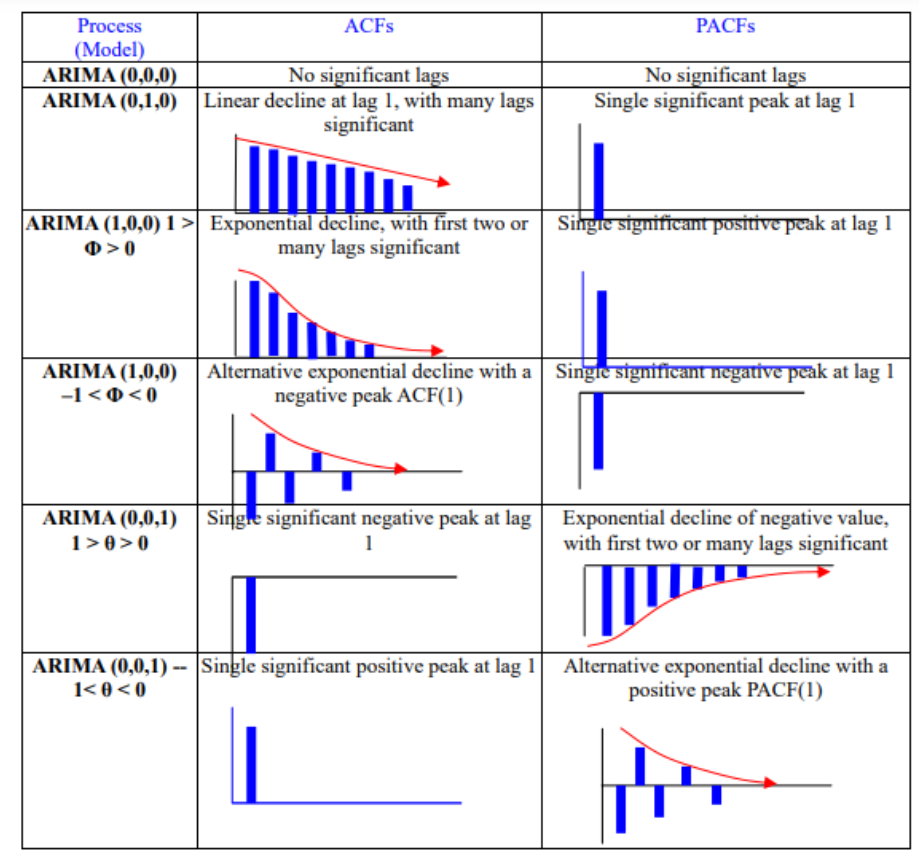
예측하기 이전에, parameter ( = p, q ) 에 따라 모형이 어떠한 모습을 띌 지 예상해봐야!
-
\(p\), \(q\) 파라미터 추론(by ACF and PACF):
- 정상성 형태 변환
- ACF & PACF 도식화
7. SARIMA(Seasonal ARIMA)
-
요약 : ARIMA + 계절성 패턴
-
형태 : Multiplicated SARIMA(p,d,q) x (P,D,Q,m)
( where \(m =\) seasonal lag of observations )
[ Summary ]
1) ARIMA(p,d,q)
\((1-\phi_1L - \cdots - \phi_p L^p) (1-L)^d Y_{t} = (1 + \theta_1 L + \cdots + \theta_q L^q) \epsilon_t\).
-
ARIMA(1,1,1)
\((1 - \phi_{1}L) (1 - L)Y_{t} = (1 + \theta_{1}L) \epsilon_{t}\).
2) SARIMA(p,d,q)\((P,D,Q)_m\)
\((1-\phi_1L - \cdots - \phi_p L^p) (1 - \Phi_{1}L^{m} - \Phi_{2}L^{2m} - \cdots - \Phi_{P}L^{Pm}) (1-L)^d (1-L^{m})^D Y_{t} =\\ (1 + \theta_1 L + \cdots + \theta_q L^q) (1 + \Theta_{1}L^{m} + \Theta_{2}L^{2m} + \cdots + \Theta_{Q}L^{Qm}) \epsilon_t\).
-
SARIMA(1,1,1)(1,1,1\()_4\)
\((1 - \phi_{1}L)~(1 - \Phi_{1}L^{4}) (1 - L) (1 - L^{4})Y_{t} = (1 + \theta_{1}L)~ (1 + \Theta_{1}L^{4})\epsilon_{t}\).
-
SARIMA(1,2,1)(1,2,1\()_4\)
\((1 - \phi_{1}L)~(1 - \Phi_{1}L^{4}) (1 - L)^2 (1 - L^{4})^2 Y_{t} = (1 + \theta_{1}L)~ (1 + \Theta_{1}L^{4})\epsilon_{t}\).
| Parameters | Description |
|---|---|
| \(p\) | Trend autoregression order |
| \(d\) | Trend difference order |
| \(q\) | Trend moving average order |
| \(m\) | the number of time steps for a single seasonal period |
| \(P\) | Seasonal autoregression order |
| \(D\) | Seasonal difference order |
| \(Q\) | Seasonal moving average order |