Classical Time Series Algorithm 4

Univariate 2. 일반 선형확률 과정 ( General Linear Process ) (2)

“시계열 데이터 = 가우시안 백색잡음의 현재값과 과거값의 선형조합”

\(Y_t = \epsilon_t + \psi_1\epsilon_{t-1} + \psi_2\epsilon_{t-2} + \cdots\).

where \(\epsilon_i \sim i.i.d.~WN(0, \sigma_{\epsilon_i}^2)~and~\displaystyle \sum_{i=1}^{\infty}\psi_i^2 < \infty\).

세부 알고리즘:

• WN(White Noise)
• MA(Moving Average)
• AR(Auto-Regressive)
• ARMA(Auto-Regressive Moving Average)
• ARMAX(ARMA with eXogenous variables)

4. ARMA(Auto-Regressive Moving Average)

\(ARMA(p,q)\): 알고리즘의 차수(\(p,q\))가 유한한 \(AR(p)\)와 \(MA(q)\)의 Linear Combination”

( 즉, \(Y_t\)는 \(Y_t\) & \(\epsilon_t\)의 차분들 (lagged variables)의 조합으로 생성 )

\[\begin{align*} Y_t = (\phi_1Y_{t-1} + \phi_2Y_{t-2} + \cdots + \phi_pY_{t-p}) + (\theta_1\epsilon_{t-1} + \theta_2\epsilon_{t-2} + \cdots + \theta_q\epsilon_{t-q}) + \epsilon_t \\ \end{align*}\]

• \(\begin{align*} where~\epsilon_i \sim i.i.d.~WN(0, \sigma_{\epsilon_i}^2)~and~\displaystyle \sum_{i=1}^{\infty}\phi_i^2 < \infty, \displaystyle \sum_{i=1}^{\infty}\theta_i^2 < \infty \end{align*}\).

위 식을 다시 정리하면…

\[\phi(L)Y_t = \theta(L)\epsilon_t\]

\(\begin{align*} Y_t &= \dfrac{\theta(L)}{\phi(L)}\epsilon_t \\ &= \psi(L)\epsilon_t \text{ where } \psi(L) = \dfrac{\theta(L)}{\phi(L)} \\ &= (1 + \psi_1L + \psi_2L^2 + \cdots)\epsilon_t \\ &= \epsilon_t + \psi_1\epsilon_{t-1} + \psi_2\epsilon_{t-2} + \cdots\end{align*}\)
where

\[\begin{aligned} \psi_1 &= \theta_1 - \phi_1 \\ \psi_2 &= \theta_2 - \phi_2 - \phi_1 \psi_1 \\ & \vdots \\ \psi_j &= \theta_j - \phi_p\psi_{j-p} - \phi_2 \psi_{p-1} - \cdots - \phi_1 \psi_{j-1} \end{aligned}\]

Autocorrelation(“Yule-Walker Equation”)

• \(\rho_i = \phi_1 \rho_{i-1} + \cdots + \phi_p \rho_{i-p}\).

[ Example ]

import pandas as pd
import numpy as np
import statsmodels
import statsmodels.api as sm
import matplotlib.pyplot as plt

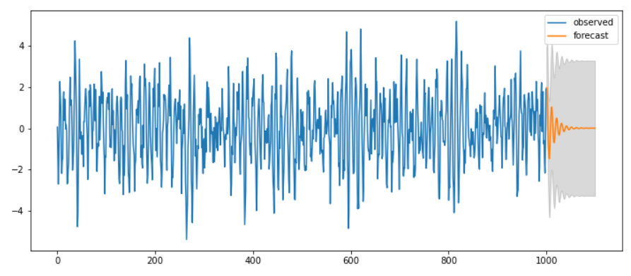
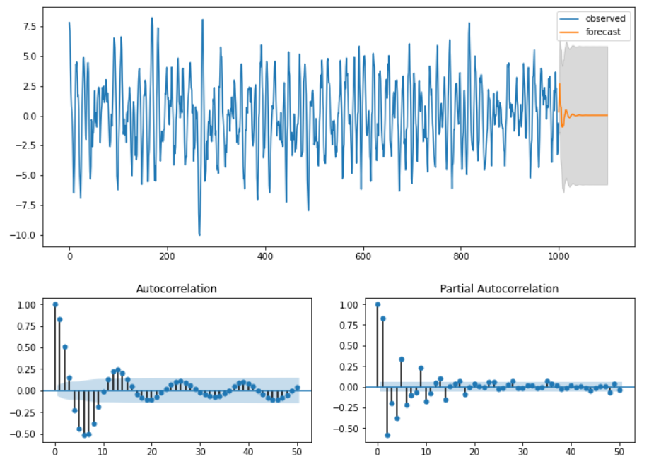
Ex 1) ARMA(2,0) = AR(2)

[Step 1] Setting

ar_params = np.array([0.75, -0.25])
ma_params = np.array([])

ar, ma = np.r_[1, -ar_params], np.r_[1, ma_params]
ar_order, ma_order = len(ar)-1, len(ma)-1

print(ar)
print(ma)
print(ar_order)
print(ma_order)
#----------------------------------------------------#
[ 1.   -0.75  0.25]
[1.]
2
0

[Step 2] Simulate data from an ARMA.

• statsmodels.tsa.arima_process.arma_generate_sample

y = statsmodels.tsa.arima_process.arma_generate_sample(ar, ma, nsample=1000, burnin=500)
y_df =pd.DataFrame(y)

[Step 3] Fit Model

• statsmodels.tsa.arima_model.ARMA
• trend='c' : constant 추가

fit = statsmodels.tsa.arima_model.ARMA(y, (ar_order,ma_order)).fit(trend='c', disp=0)

[Step 4] Forecast Result

ahead = 100
pred_ts_point = fit.forecast(steps=ahead)[0]
pred_ts_interval = fit.forecast(steps=ahead)[2]

print(pred_ts_point.shape)
print(pred_ts_interval.shape) # default : alpha=0.05
print(pred_ts_point[0]==np.mean(pred_ts_interval[0]))

#----------------------------------------------------#
(100,)
(100, 2)
True

forecast_index :

• 예측하려는 대상의 time

• 1000 ~ 1000+ahead(=1100)

forecast_index = [i for i in range(y_df.index.max()+1,y_df.index.max()+ahead+1)]

pred_point_df=pd.DataFrame(pred_ts_point, index=forecast_index)
pred_interval_df = pd.DataFrame(pred_ts_interval, index=forecast_index)

print(pred_point_df.head())
print(pred_interval_df.head())

#----------------------------------------------------#
             0
1000  1.971779
1001  1.940186
1002  1.492918
1003  0.058082
1004 -0.935687
             0         1
1000  0.093410  3.850149
1001 -0.404395  4.284767
1002 -0.921029  3.906864
1003 -2.385855  2.502019
1004 -3.433020  1.561645

[Step 5] Result

main_plot = y_df.plot(figsize=(12,5))
pred_point_df.plot(label='forecast', ax=main_plot)

main_plot.fill_between(pred_interval_df.index,
                pred_interval_df.iloc[:,0],pred_interval_df.iloc[:,1], 
                color='k', alpha=0.15)
plt.legend(['observed', 'forecast'])

display(fit.summary2())

Model:	ARMA	BIC:	2796.4388
Dependent Variable:	y	Log-Likelihood:	-1377.5
Date:	2021-09-01 12:20	Scale:	1.0000
No. Observations:	1000	Method:	css-mle
Df Model:	5	Sample:	0
Df Residuals:	995		0
Converged:	1.0000	S.D. of innovations:	0.958
No. Iterations:	12.0000	HQIC:	2778.184
AIC:	2766.9923

	Coef.	Std.Err.	t	P>|t|	[0.025	0.975]
const	0.0093	0.0374	0.2500	0.8026	-0.0639	0.0826
ar.L1.y	0.7470	0.0279	26.7627	0.0000	0.6923	0.8017
ar.L2.y	-0.2521	0.0362	-6.9600	0.0000	-0.3231	-0.1811
ar.L3.y	0.1631	0.0362	4.4995	0.0000	0.0920	0.2341
ar.L4.y	-0.4699	0.0279	-16.8256	0.0000	-0.5247	-0.4152

	Real	Imaginary	Modulus	Frequency
AR.1	0.8756	-0.6261	1.0764	-0.0988
AR.2	0.8756	0.6261	1.0764	0.0988
AR.3	-0.7021	-1.1592	1.3553	-0.3367
AR.4	-0.7021	1.1592	1.3553	0.3367

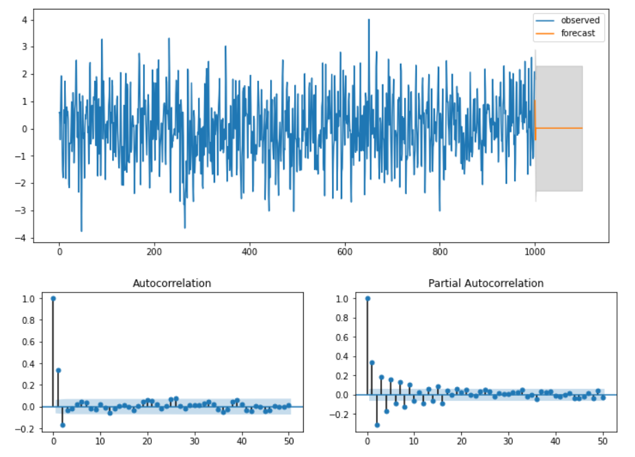
plt.figure(figsize=(12,3))
statsmodels.graphics.tsaplots.plot_acf(y, lags=50, zero=True, use_vlines=True,
                                       alpha=0.05, ax=plt.subplot(121))
statsmodels.graphics.tsaplots.plot_pacf(y, lags=50, zero=True, use_vlines=True, 
                                        alpha=0.05, ax=plt.subplot(122))
plt.show()

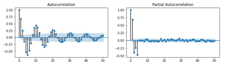
Ex 2) ARMA(0,2) = MA(2)

ar_params = np.array([])
ma_params = np.array([0.65, -0.25])

Model:	ARMA	BIC:	2783.1398
Dependent Variable:	y	Log-Likelihood:	-1377.8
Date:	2020-09-29 23:34	Scale:	1.0000
No. Observations:	1000	Method:	css-mle
Df Model:	3	Sample:	0
Df Residuals:	997		0
Converged:	1.0000	S.D. of innovations:	0.959
No. Iterations:	8.0000	HQIC:	2770.970
AIC:	2763.5088

	Coef.	Std.Err.	t	P>|t|	[0.025	0.975]
const	0.0130	0.0425	0.3053	0.7602	-0.0703	0.0962
ma.L1.y	0.6501	0.0310	20.9416	0.0000	0.5892	0.7109
ma.L2.y	-0.2487	0.0307	-8.0906	0.0000	-0.3090	-0.1885

	Real	Imaginary	Modulus	Frequency
MA.1	-1.0865	0.0000	1.0865	0.5000
MA.2	3.7001	0.0000	3.7001	0.0000

Ex 3) ARMA(1,1)

ar_params = np.array([0.75])
ma_params = np.array([0.65])

Model:	ARMA	BIC:	2783.7601
Dependent Variable:	y	Log-Likelihood:	-1378.1
Date:	2020-07-31 22:45	Scale:	1.0000
No. Observations:	1000	Method:	css-mle
Df Model:	3	Sample:	0
Df Residuals:	997		0
Converged:	1.0000	S.D. of innovations:	0.959
No. Iterations:	9.0000	HQIC:	2771.590
AIC:	2764.1291

	Coef.	Std.Err.	t	P>|t|	[0.025	0.975]
const	0.0641	0.1970	0.3252	0.7450	-0.3220	0.4501
ar.L1.y	0.7465	0.0224	33.3502	0.0000	0.7027	0.7904
ma.L1.y	0.6519	0.0261	24.9637	0.0000	0.6007	0.7031

	Real	Imaginary	Modulus	Frequency
AR.1	1.3395	0.0000	1.3395	0.0000
MA.1	-1.5340	0.0000	1.5340	0.5000

Ex 4) ARMA(5,5)

ar_params = np.array([0.75, -0.25, 0.5, -0.5, -0.1])
ma_params = np.array([0.65, 0.5, 0.2, -0.5, -0.1])

Model:	ARMA	BIC:	2844.4865
Dependent Variable:	y	Log-Likelihood:	-1380.8
Date:	2020-09-29 23:41	Scale:	1.0000
No. Observations:	1000	Method:	css-mle
Df Model:	11	Sample:	0
Df Residuals:	989		0
Converged:	1.0000	S.D. of innovations:	0.959
No. Iterations:	54.0000	HQIC:	2807.977
AIC:	2785.5934

	Coef.	Std.Err.	t	P>|t|	[0.025	0.975]
const	0.0308	0.0864	0.3569	0.7212	-0.1386	0.2003
ar.L1.y	1.3387	0.4949	2.7049	0.0068	0.3687	2.3087
ar.L2.y	-0.7833	0.4780	-1.6387	0.1013	-1.7202	0.1536
ar.L3.y	0.7138	0.2246	3.1786	0.0015	0.2737	1.1540
ar.L4.y	-0.7757	0.2729	-2.8428	0.0045	-1.3106	-0.2409
ar.L5.y	0.2339	0.2687	0.8705	0.3840	-0.2927	0.7604
ma.L1.y	0.0678	0.4967	0.1366	0.8914	-0.9057	1.0413
ma.L2.y	0.2093	0.2164	0.9674	0.3334	-0.2148	0.6334
ma.L3.y	-0.0514	0.1982	-0.2592	0.7955	-0.4398	0.3371
ma.L4.y	-0.6159	0.0713	-8.6358	0.0000	-0.7557	-0.4762
ma.L5.y	0.1658	0.2752	0.6026	0.5467	-0.3735	0.7052

	Real	Imaginary	Modulus	Frequency
AR.1	-0.4994	-1.1024	1.2103	-0.3177
AR.2	-0.4994	1.1024	1.2103	0.3177
AR.3	1.0036	-0.5072	1.1245	-0.0745
AR.4	1.0036	0.5072	1.1245	0.0745
AR.5	2.3086	-0.0000	2.3086	-0.0000
MA.1	-1.1194	-0.0000	1.1194	-0.5000
MA.2	-0.0971	-1.0335	1.0381	-0.2649
MA.3	-0.0971	1.0335	1.0381	0.2649
MA.4	1.3648	-0.0000	1.3648	-0.0000
MA.5	3.6628	-0.0000	3.6628	-0.0000

모형 차수결정 정리

• 예측하기 이전에, parameter ( = p, q ) 에 따라 모형이 어떠한 모습을 띌 지 예상해봐야!
• \(p\), \(q\) 파라미터 추론(by ACF and PACF):
  • 정상성 형태 변환
  • ACF​ & PACF 도식화

	자기회귀: \(AR(p)\)	이동평균: \(MA(q)\)	자기회귀이동평균: \(ARMA(p,q)\)
\(ACF\)	지수적 감소, 진동하는 sine 형태	\(q+1\) 차항부터 절단모양(0수렴)	\(q+1\) 차항부터 지수적 감소 혹은 진동하는 sine 형태
\(PACF\)	\(p+1\) 차항부터 절단모양(0수렴)	지수적 감소, 진동하는 sine 형태	\(p+1\) 차항부터 지수적 감소 혹은 진동하는 sine 형태

5. ARMAX ( ARMA with eXogenous)

ARMA에 \(\beta X\) 가 추가된 형태

ARMA 식

• \(Y_t = \phi_1Y_{t-1} + \phi_2Y_{t-2} + \cdots + \phi_pY_{t-p} + \theta_1\epsilon_{t-1} + \theta_2\epsilon_{t-2} + \cdots + \theta_q\epsilon_{t-q} + \epsilon_t\).

ARMAX 식

• \(Y_t = \phi_1Y_{t-1} + \phi_2Y_{t-2} + \cdots + \phi_pY_{t-p} + \theta_1\epsilon_{t-1} + \theta_2\epsilon_{t-2} + \cdots + \theta_q\epsilon_{t-q} + \epsilon_t + \beta X\).

[ Example ]

Seasonal ARMAX : sm.tsa.SARIMAX

fit = sm.tsa.SARIMAX(raw_using.consump, exog=raw_using.m2, 
                     order=(1,0,0), seasonal_order=(1,0,1,4)).fit()

6. ARMAX ( ARMA with eXogenous)