Unsupervised feature learning for audio classification using convolutional deep belief networks (NeurIPS 2009)
http://www.robotics.stanford.edu/~ang/papers/nips09-AudioConvolutionalDBN.pdf
Contents
- Abstract
- Introduction
- Unsupervised Feature Learning
- Application to speech recognition tasks
- Application to music classification tasks
0. Abstract
Apply convolutional deep belief networks to audio data
& evaluate them on various audio classification tasks
1. Introduction
DL have not been extensively applied to auditory data.
Deep belief network
- generative probabilistic model
- composed of one visible (observed) layer and many hidden layers
- can be efficiently trained using greedy layerwise training
We will apply convolutional deep belief networks to unlabeled auditory data
\(\rightarrow\) outperform other baseline features (spectrogram and MFCC)
Phone classification task
- MFCC features can be augmented with our features to improve accuracy
2. Unsupervised Feature Learning
Training on unlabeled TIMIT data
TIMIT: large, unlabeled speech dataset
- step1) extract the spectrogram from each utterance of the TIMIT training data
- spectrogram = 20 ms window size with 10 ms overlaps
- spectrogram was further processed using PCA whitening (with 80 components)
- step 2) train model
3. Application to speech recognition tasks
CDBN feature representations learned from the unlabeled speech corpus can be useful for multiple speech recognition tasks
- ex) speaker identification, gender classification, and phone classification
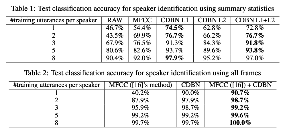
(1) Speaker identification
The subset of the TIMIT corpus
- 168 speakers and 10 utterances (sentences) per speake ( = total of 1680 utterances )
\(\rightarrow\) 168-way classification
Extracted a spectrogram from each utterance
- spectrogram = “RAW” features.
- first and second-layer CDBN features using the spectrogram as input
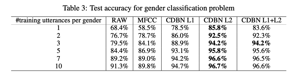
(2) Speaker gender classification
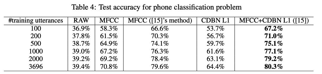
(3) Phone classification
treat each phone segment as an individual example
compute the spectrogram (RAW) and MFCC features for each phone segment.
- 39 way phone classification accuracy on the test data for various numbers of training sentences
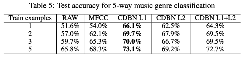
4. Application to music classification tasks
(1) Music genre classification
Dataset
-
unlabeled collection of music data.
- computed the spectrogram representation for individual songs
- 20 ms window size with 10 ms overlaps)
- spectrogram was PCA-whitened
Task: 5 way genre classification tasks: (classical, electric, jazz, pop, and rock)
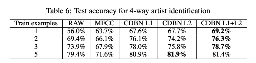
(2) Music artist classification
4 way artist classification task