AST; Audio Spectrogram Transformer

AST: Audio Spectrogram Transformer ( arxiv 2021 )

https://arxiv.org/pdf/2104.01778.pdf

Contents

1. Abstract
2. Introduction
3. AST
   1. Model Architecture
   2. ImageNet Pretraining
4. Experiments
   1. AudioSet Experiments
   2. Results on ESC-50 & Speech Commands

Abstract

To better capture long-range global context…

\(\rightarrow\) add a self-attention mechanism

However, it is unclear whether the reliance on a CNN is necessary

Audio Spectrogram Transformer (AST)

the first convolution-free, purely attention-based model for audio classification

1. Introduction

Audio Spectrogram Transformer (AST),

• a convolution-free, purely attentionbased model
• directly applied to an audio spectrogram
• capture long-range global context even in the lowest layers.
• (Additional) approach for transferring knowledge from the Vision Transformer (ViT) [12] pretrained on ImageNet [14] to AST,

Advantages of AST

• (1) superior performance
  • evaluate on a variety of audio classification tasks and datasets including AudioSet [15], ESC-50 [16] and Speech Commands [17].
• (2) variable-length inputs & can be applied to different tasks without any change of architecture.
• (3) features a simpler architecture with fewer parameters, and converges faster during training.

Related Work: Vision Transformer (ViT)

• AST and ViT have similar architectures, but the difference is…
  • ViT : has only been applied to fixed-dimensional inputs (images)
  • AST : can process variable-length audio inputs.
• propose an approach to transfer knowledge from ImageNet pretrained ViT to AST

2. AST

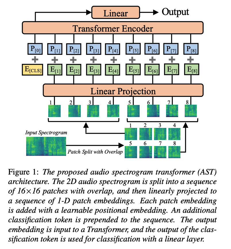
(1) Model Architecture

a) Procedure

Step 1) Convert to Melspectogram

• Input audio waveform of \(t\) seconds \(\rightarrow\) sequence of 128-dim log Mel filterbank (fbank) features
  • omputed with a 25ms Hamming window every 10ms.
• Result : 128×100\(t\) spectrogram ( = input to AST )

Step 2) Patching

• split the spectrogram into a sequence of \(N\) 16×16 patches with an overlap of \(6\) in both time and frequency dimension
• number of pacthes \(N=12\lceil(100 t-16) / 10\rceil\)

Step 3) Flatten ( using a linear projection layer )

• each \(16 \times 16\) patch \(\rightarrow\) \(1 D\) patch embedding of size 768
• also called patch embedding layer

Step 4) Trainable positional embedding

• \(\because\) Transformer does not capture the input order information & and the patch sequence is also not in temporal order
• ( + append a [CLS] token at the beginning of the sequence )

b) Architecture

• Transformer: consists of several encoder and decoder layers

  \(\rightarrow\) only use the ENCODER of the Transformer.

  ( \(\because\) AST is designed for classification tasks )

• use the original Transformer encoder [18] architecture without modification
  • Advantages of this simple setup :
    • (1) easy to implement and reproduce as it is off-the-shelf in TensorFlow and PyTorch
    • (2) intend to apply transfer learning for AST, and a standard architecture makes transfer learning easier
• Transformer encoder’s output of the [CLS] token serves as the audio spectrogram representation
• Linear layer with sigmoid activation maps the audio spectrogram representation to labels for classification.

Is it truly convolution-free?

• Patch Embedding Layer

  = can be viewed as a single convolution layer with a large kernel and stride size

• Projection layer in each Transformer block

  = equivalent to \(1 \times 1\) convolution.

\(\rightarrow\) However, the design is different from conventional CNNs that have multiple layers and small kernel and stride sizes

\(\rightarrow\) Thus usually referred to as convolution-free

(2) ImageNet Pretraining

Disadvantage of the Transformer ( compared with CNNs )

= needs more data to train!

\(\rightarrow\) However, audio datasets typically do not have such large amounts of data

\(\rightarrow\) motivates us to apply cross-modality transfer learning to AST

• since images and audio spectrograms have similar formats.

Solution: adapting an off-the-shelf pretrained Vision Transformer (ViT) to AST

Difference btw ViT & AST

(1) # of input channel

• ViT = 3 \(\leftrightarrow\) AST = 1
• solution: average the weights corresponding to each of the 3 input channels
• also normalize the input audio spectrogram so that the dataset mean and standard deviation are 0 and 0.5

(2) input shape

• ViT : fixed (either 224×224 or 384 × 384)

• AST: length of an audio spectrogram can be variable.

  \(\rightarrow\) positional embedding needs to be carefully processed

  • propose a cut and bi-linear interpolate method for positional embedding adaptation
  • directly reuse the positional embedding for the [CLS] token.

(3) Downstream Task

• classification task is essentially different!
• solution : abandon the last classification layer of the ViT and reinitialize a new one for AST

With this adaptation framework, the AST can use various pretrained ViT weights for initialization.

• (in this work) use pretrained weights of a data-efficient image Transformer (DeiT)
  • DeiT has two [CLS] token \(\rightarrow\) average them as a single [CLS] token for audio training.

3. Experiments

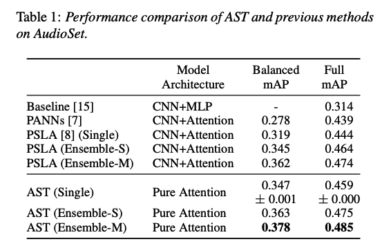
(1) AudioSet Experiments

AudioSet

• weakly-labeled audio event classification
• one of the most challenging audio classification tasks.

a) Dataset and Training Details

AudioSet

• collection of over 2 million 10-second audio clips excised from YouTube videos
• labeled with the sounds that the clip contains from a set of 527 labels.
• size : ( balanced training, full training, and evaluation set ) = ( 22k, 2M, 20k )

Same training pipeline with [8]

b) Results

c) Ablation Study

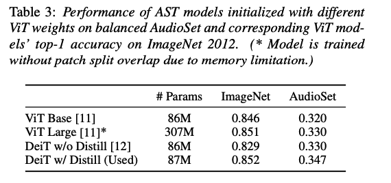
[Impact of ImageNet Pretraining]

performance improvement:

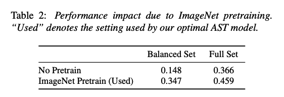
impact of pretrained weights used

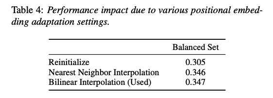
[Impact of Positional Embedding Adaptation]

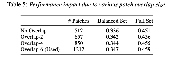
[Impact of Patch Split Overlap]

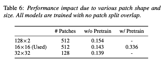
[Impact of Patch Shape and Size]

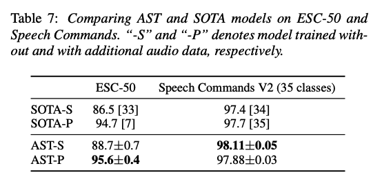
(2) Results on ESC-50 & Speech Commands

ESC-50 [16]

• consists of 2,000 5-second environmental audio recordings organized into 50 classes

Speech Commands V2 [17]

• consists of 105,829 1-second recordings of 35 common speech commands.