Masked Autoencoders that Listen

Masked Autoencoders that Listen (NeurIPS 2022)

https://arxiv.org/pdf/2207.06405.pdf

Contents

1. Abstract
2. Introduction
3. Related Work
   1. Visual masked pre-training
   2. Out-of-domain pre-training for audio
   3. In-domain pretraining for aduio
4. Audio-MAE
   1. Spectogram Patch Embeddings
   2. Masking strategies
   3. Encoder
   4. Decoder with Local Attention
   5. Objective
   6. Fine-tuning for Downstream Tasks
5. Experiments
   1. Datasets and Tasks
   2. Implementation Details
   3. Pre-training and Fine-tuning
   4. Ablations and Model properties
   5. Comparion with SOTA
   6. Visualization

0. Abstract

Masked Autoencoders (MAE) for audio spectrograms

• Transformer encoder-decoder design

• [1] Pretrain

  • Encoder

    • (1) encode audio “spectrogram patches” with a HIGH masking ratio
    • (2) feed only the NON-masked tokens through encoder layers.

  • Decoder

    • (3) re-ordes and decode the encoded context padded with mask tokens

      ( + beneficial to incorporate local window attention in the decoder, as audio spectrograms are highly correlated in local time and frequency bands )

• [2] Fine-tune : with a LOWER masking ratio on target datasets.

• Experiments: new SOTA performance on six audio and speech classification tasks

1. Introduction

Masked Autoencoders (MAE)

Transformer-based models : SOTA for audio understanding tasks.

• AST [10] and MBT [11] :

  • improved the audio classification performance on the AudioSet [12], Event Sound Classification [13], etc.

  • key technique = initialization of audio model weights with “ImageNet” pre-trained supervised models

    • by deflating patch embeddings and interpolating positional embeddings for encoding audio spectrograms.

    \(\rightarrow\) However, exploiting ImageNet pre-trained models could be sub-optimal !!

    ( \(\because\) discrepancies between spectrograms representing audio content and natural images )

Solution: Self-supervised audio representation learning

• SS-AST [18]
  • based on BEiT [17] that learns to reconstruct image patches or learnt patch tokens
    • extends to the audio domain and exploits spectrograms (akin to 1-channel 2D images)
  • Two loss functions for SSL
    • (1) contrastive loss
    • (2) reconstruction loass
  • utilize large-scale pre-training data

Experiment: use AudioSet [12] for pre-training

• a common dataset containing ∼2 million audio recordings

• However, performing large-scale training with Transformer architectures is challenging !

  ( \(\because\) *quadratic complexity8 w.r.t. the length of input sequence )

Solution for complexity: reduce the sequence length in self-attention

• various ViT-based architectures have been developed to alleviate
  • Swin-Transformer [19] : only performs local attention within windows that shift across layers.
  • MViT [20] : employs pooling attention to construct a hierarchy of Transformers where sequence lengths are downsampled.
  • MAE [1] : efficiently encodes only a small portion (25%) of visual patches while the majority of patches is discarded.
    • The simplicity and scalability in MAE make it a promising framework for large-scale SSL

AudioMAE

• unified and scalable framework for learning SSL audio representations

• for sound recognition and the unique challenges of the audio domain

• composed of a pair of a Transformer encoder and decoder

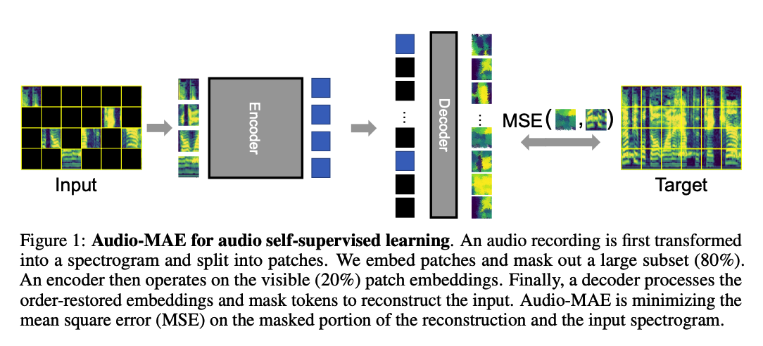
Procedures of AudioMAE

• (1) sound \(\rightarrow\) spectrogram patches.

• (2) Encoding

  • mask & discard the majority ( = only feed a small number of NON-masked embeddings )

    \(\rightarrow\) for efficient encoding.

• (3) Decoding

  • Input : (a) Encoded patches + (b) Learnable embeddings ( = representing masked patches )
  • Restores the order of these patches in frequency and time
  • Propagates them through a decoder to reconstruct the audio spectrogram

Image vs. Spectrogram

Spectrogram patches are comparably local-correlated

• ex) formants ( the vocal tract resonances ) are typically grouped and continuous locally in the spectrogram.
• The location in frequency and time embeds essential information that determines the semantics of a spectrogram patch and how it sounds like.

\(\rightarrow\) we further investigate using (1) localized attention and a (2) hybrid architecture in the Transformer decoder to properly decode for reconstruction.

\(\rightarrow\) improved performance for Audio-MAE.

Experiments

SOTA performance on six audio and speech classification tasks.

• first audio-only SSL model that achieves state-of-the-art mAP on AudioSet-2M
• visualization & audible examples to qualitatively demonstrate the effectiveness of the Audio-MAE decoder

2. Related Work

(1) Visual masked pre-training

BEiT [17] and MAE [1]

• based on ViT [9] that applies Transformers to image patches,
• BEiT [17] : learns to predict discrete visual tokens generated by VAE [25] in masked patches.
• MAE [1] : reduces sequence length by masking a large portion of image patches randomly and encoding ONLY non-masked ones for reconstruction of pixel color information.

MaskFeat [20]

• studies features for masked pre-training and finds that Histograms of Oriented Gradients (HoG) [26]
  • related to spectrogram features
• perform strongly for image and video classification models.

(2) Out-of-domain pre-training for audio

Transferring ImageNet supervised pre-trained ViT [9] or ResNet [27]

\(\rightarrow\) has become a popular practice for audio models [10, 28, 11, 29, 30, 31].

Fine-tuning to audio

• to audio spectrograms
  • from 3-channels (RGB) into **1-channel (spectrogram) **
• employing the rest of the transformer blocks on top.

HTS-AT [29] : encodes spectrograms with hierarchical Transformer initialized from the Swin Transformer

MBT [11] : uses ImageNet-21K pre-trained ViT

AST [10], PaSST [28] : employ DeiT [14] as the Transformer backbone.

Without using out-of-domain (non-audio) data…

\(\rightarrow\) Audio-MAE focuses on AUDIO-ONLY SSL pre-training from scratch

(3) In-domain pre-training for audio

Categorized by the (1) input signal type

• raw waveform [32, 33, 34]
• frame-level features [35, 36, 37]
• spectrogram patches [18, 38]

Categorized by the (2) objective used for self-supervision

• contrastive [39, 33, 40, 41, 35]
• prediction/reconstruction [18, 34, 37, 36]

wav2vec 2.0 [33] :

• [input] RAW waveform
• [train] contrastive learning
  • to discriminate contextualized representations in different time segments.

Mockingjay [42] :

• proposed a masked acoustic model pretext task to reconstruct frame-level Mel-features of masked time frames.

SSAST [18] :

• closest work to Audio-MAE & main benchmark.

SS-AST :

• Inspired by the success of BERT [3],
• SSL method which operates over spectrogram patches
• [train] both contrastive and reconstructive objectives

\(\rightarrow\) these previous methods generate audio representations by encoding FULL-view of both masked and nonmasked time or spectrogram segments for self-supervised pre-training.

\(\leftrightarrow\) Audio-MAE encodes only the non-masked spectrogram patches.

Concurrent work : [38,43,44]

3. Audio-MAE

(1) Spectrogram Patch Embeddings

Step 1) Transform audio recordings into Melspectrograms

Step 2) Divide them into non-overlapped regular grid patches.

Step 3) Flattened

Step 4) Embedded by a linear projection.

( + add fixed sinusoidal positional embeddings to the embedded patches )

(2) Masking strategies

Masking mechanism is the key ingredient for efficient SSL

masks out a large subset of spectrogram patches

• can be viewed as a 2D representation of time and frequency components of a sound

  \(\rightarrow\) reasonable to explore treating time and frequency differently during masking.

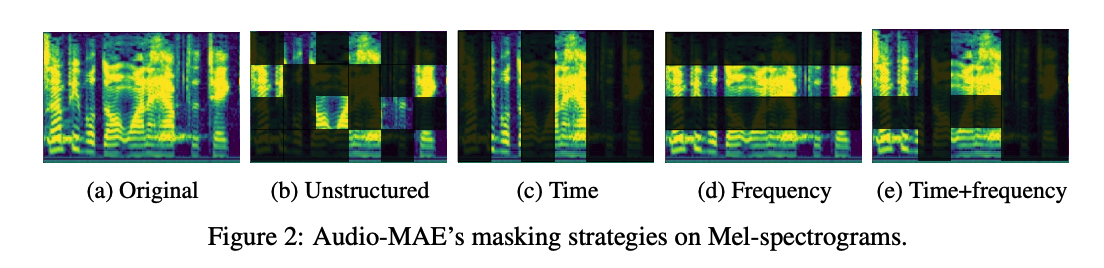
investigate both the unstructured & structured

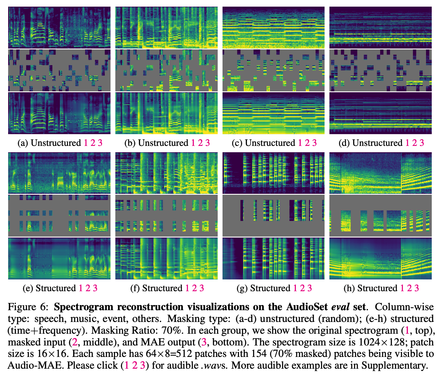
• (1) unstructured: random masking without any prior
• (2) structured: randomly masking a portion of time, frequency, or time+frequency of a spectrogram

Masking Ratio: large masking rate

• AudioMAE: 80%
• original MAE : 75%
• BERT : 15%

\(\rightarrow\) Audio MAE & original MAE : most of the tokens/patches can be discarded due to high redundancy

Empirically found that

• pretraining = unstructured (random) masking at a higher ratio
• fine-tuning = structured (time+frequency) masking at a lower ratio

(3) Encoder

• Stack of standard Transformers
  • (default) 12-layer ViT-Base (ViT-B) [9]
• only processes (20%) non-masked patches to reduce computation overhead

(4) Decoder with Local Attention

• Standard Transformer blocks
• input = (1) + (2)
  • [ UN-MASKED ] : (1) encoded patches from the encoder
  • [ MASKED ] : (2) trainable masked tokens
• After restoring the original time-frequency order in the audio spectrogram…
  • (1) add the decoder’s (fixed sinusoidal) positional embeddings
  • (2) feed the restored sequence into the decoder.
• add a linear head for reconstruction

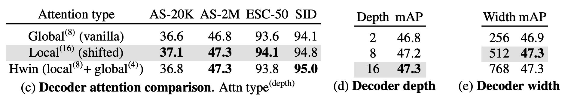
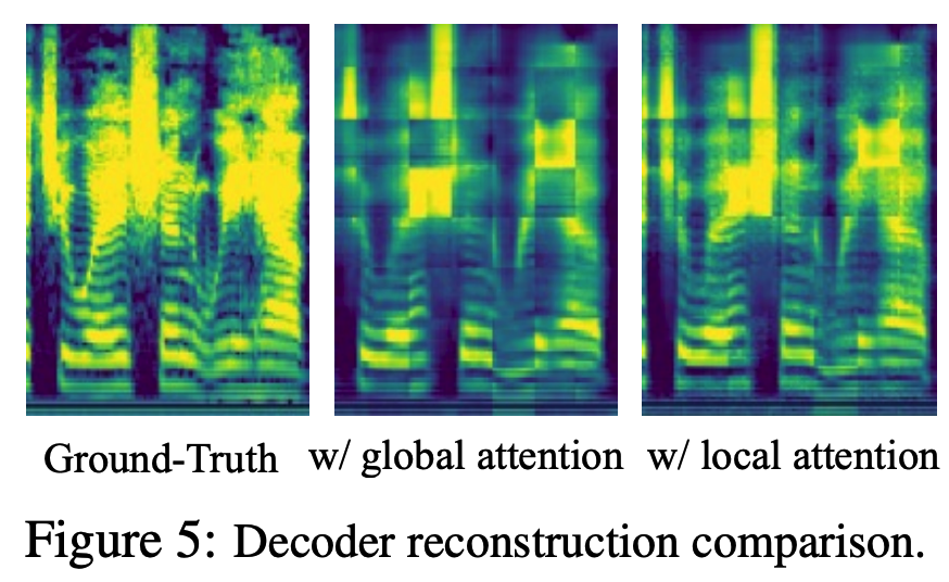
Image-based MAE

uses global self-attention in the Transformer decoder which is appropriate for visual context

(\(\because\) because visual objects are typically invariant under translation or scaling, and their exact position may not affect the semantics of an image )

Audio MAE

the position, scale, and translation of spectrogram features directly affects the sound or semantics of an audio recording.

\(\rightarrow\) global self-attention is sub-optimal for spectrograms, if the time-frequency components is predominantly local

Compared to images, the spectrogram patches are more similar to speech or text tokens

\(\because\) where its order and position is more relevant

Solution: incorporate the LOCAL attention mechanism

• which groups and separates the spectrogram patches in to LOCAL windows in self-attention for decoding.
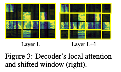
• investigate two types of local attention:
  • (1) Shifted window location (Figure 3)
    • inspired by the shifted-window in Swin Transformers
    • shift window attention by 50% between consecutive Transformer decoder layers.
    • for padding the margin when shifting, we cyclically shift the spectrogram to the top-left direction
  • (2) Hybrid window attention (global+local attention)
    • to add better cross-window connections
    • design a simple hybrid (global+local) attention that computes local attention within a window in all but the last few top layers.
    • input feature maps for the final reconstruction layer also contain global information. F
• for simplicity, we use no pooling or hierarchical structure

(5) Objective

Goal: reconstruct the input spectrogram

Loss: mean squared error (MSE)

• between the prediction and the input spectrogram, averaged over unknown patches.

via Experiments: employing the reconstruction loss ALONE is sufficient

• ( including additional contrastive objectives does not improve Audio-MAE. )

(6) Fine-tuning for Downstream Tasks

• Only keep and fine-tune the AudioMAE encoder and discard the decoder

• explore to employ masking in the fine-tuning stage to remove a portion of patches to further regularize learning from a limited view of spectrogram inputs, which, as a side effect, also reduces computation during fine-tuning.

SpecAug [48] vs. Audio-MAE

• SpecAug: takes full-length input with the masked portion set to zero as data augmentation
• Audio-MAE: sees only a subset of real-valued input patches without the nullified ones.
  • encodes these non-masked patches
  • applies an average pooling layer followed by a linear layer on top for fine-tuning in classification tasks.

4. Experiments

Extensive evaluation on six tasks

• (1) Audio classification on AudioSet (AS-2M, AS-20K)
  • also for ablation study
• (2) Environmental Sound Classification (ESC-50)
• (3) Speech classification on Speech Commands (SPC-1 and SPC-2) and VoxCeleb (SID).

(1) Datasets and Tasks

AudioSet [12] (AS-2M, AS-20K)

• ∼2 million 10-second YouTube clips for audio classification

• 527 types of audio events are weakly annotated [49, 50, 51] for each clip.

  ( could be multiple events in a clip )

• Full training set has 2 subsets:
  • (1) Class-wise balanced (22,176 clips)
  • (2) Unbalanced (2,042,985 clips) set.
• Eval set : 20,383 clips.
• Preprocessed ….
  • Train:
    • 1.96M unbalanced training
    • 21K balanced training evaluation clips
  • Eval:
    • 19K evaluation clips
• AS-2M experiments
  • [pretrain & finetune] union of unbalanced and balanced training audio
• AS-20K experiments
  • [pretrain] AS-2M
  • [finetune] 20K balanced set
• Test result: mAP on the 19K eval set

Environmental Sound Classification (ESC-50) [13]

• Audio classification dataset
• 2,000 5-second environmental sound recordings.
• # of class = 50
• accuracy under 5-fold cross-validation with the same split used by [10].

Speech Commands (SPC-2, SPC-1) [52]

Two keyword spotting tasks.

• SPC-2 : 35 speech commands
  • (training/validation/testing) set = (84,843/9,981/11,005) 1-second recordings
• SPC-1 : 10 classes of keywords
  • 1 silence class, and 1 unknown class that includes all the other 20 common speech commands.
• use the data and split provided in the SUPERB [53] benchmark to report the testing accuracy.

VoxCeleb (SID) [54]

• Speaker identification task (SID)
  • classify the utterances to identify its original speaker.
• 150K utterances from 1,251 speakers
• use the standard train (138,361), validation (6,904), testing (8,251) sets
• report testing accuracy

(2) Implementation Details

Architecture

• Encoder: vanilla 12-layer ViT-B

• Decoder: 16-layer Transformer with shifted local attention

Data preprocessing

• transform raw waveform **(pre-processed as mono channel under 16,000 sampling rate) into **Mel-frequency bands with a 25ms Hanning window that shifts every 10 ms.
• ex) For a 10-second recording in AudioSet, the resulting spectrogram is of 1×1024×128 dimension

Patch embedding :

• convolutional kernels with (16, 16) size and stride in time and frequency (thus, patches are non-overlapping) to avoid short-cuts via overlap in self-supervision

Masking strategies

• [pre-training] Masking ratio of 0.8 with (unstructured) random masking
• [fine-tuning] Masking ratio of 0.3

(3) Pre-training and Fine-tuning

Pretraining

• dataset: AudioSet-2M

• 32 epochs with a batch size of 512 and a 0.0002 learning rate

• distribute the training load over 64 V100 GPUs and the total training time is ∼36 hours.

• For each audio, we randomly sample the starting time, cyclically extract 10-second audio, and randomly jitter its magnitude by up to ± 6dB.

• use only natural audio spectrograms a ( No augmentations )

  • do not find these strong augmentations helpful in the pre-training phase.

Fine-tuning phase

• only fine-tune the encoder ( remove decoder )

• 100 epochs

  • each epoch = sample 200K instances (∼10% of AudioSet-2M) without replacement.

• (For supervised fine-tuning on AudioSet-2M)

  • # of training samples are uneven across classes (unbalanced) \(\rightarrow\) weighted sampling
    • weight = inversely proportional to the dataset-wise occurrences of its classes.

• Fine-tuning on 64 GPUs takes ∼12 hours.

  ( For the smaller balanced AudioSet-20K, we fine-tune on 4 GPUs for 60 epochs without weighted sampling. Please see Supplementary for the details on other datasets. )

(4) Ablations and Model Properties

a) Masking Strategies in Pre-training & Fine-tuning

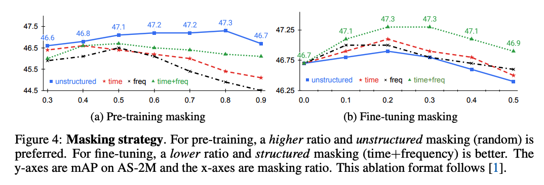
[Findings]

1. [Pretraining] HIGH pre-training masking ratio (80% in our case) is optimal!
   • both audio spectrograms and images are continuous signals with significant redundancy.

2. [Pretraining] Unstructured random masking works the best!

   • Unlike MAE for images, there are clear performance differences among masking strategies!

3. [Pretraining] For higher masking ratios, the structured masking alternatives drop in performance

   • presumably because the task becomes too difficult while random masking improves steadily up to 80%.

   • show that designing a pretext task with proper hardness is important for effective

   \(\rightarrow\) use random masking with ratio of 80% as our default for pre-training.

4. [Fine-tuning] Use structured masking:
   • time+frequency > time- or frequency-based masking > unstructured masking.
   • optimal masking ratios are lower than for pre-training

b) Impact of Patch Size and Stride

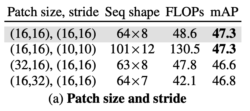
• Previous Works
  • following AST, use overlapped patches (patch = 16 and stride = 10) to boost end task performance.
• Audio-MAE
  • do not observe a performance improvement using overlapped patches ( due to leakage in information )
  • non-overlapped 16×16 patches achieve a good balance between computation and performance

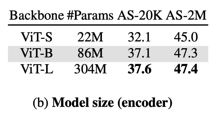
c) Encoder

d) Decoder

e) Pre-training Data and Setup

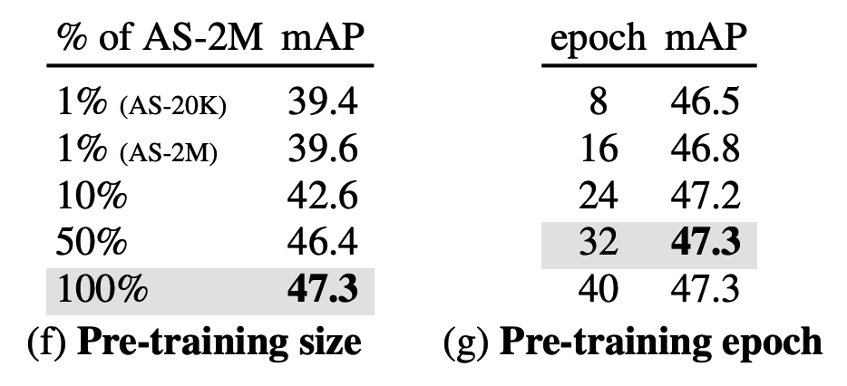
Impact of pre-training dataset size: (1) vs (2)

• (1) 1% well-annotated AS-20K balanced data
• (2) randomly sampled 20K unbalanced data

\(\rightarrow\) similar mAPs (39.4 vs 39.6) …. suggest that the distribution of data classes (balanced vs. unbalanced) is less important for pre-training.

Training for longer is beneficial yet the performance saturates after the 24-th epoch

f) Out-of-domain Pre-training on ImageNet

Significant discrepancies between image and audio modalities

\(\rightarrow\) questionable if out-of-domain pre-training benefits audio representation learning.

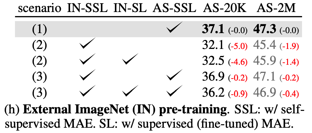
3 scenarios

• (1) Audio-only pre-training (AS-SSL) from scratch.
  • ideal schema for learning audio representations
  • prevents uncontrollable bias transfer from other modalities
• (2) Directly using SSL ImageNet MAE models (IN-SSL) and its fine-tuned variant (IN-SL).
• (3) Audio-MAE SSL pre-training on top of these ImageNet weights.

\(\rightarrow\) out-of-domain pre-training (i.e., ImageNet) is not helpful for Audio-MAE, possibly due to domain shift

(5) Comparison with SOTA

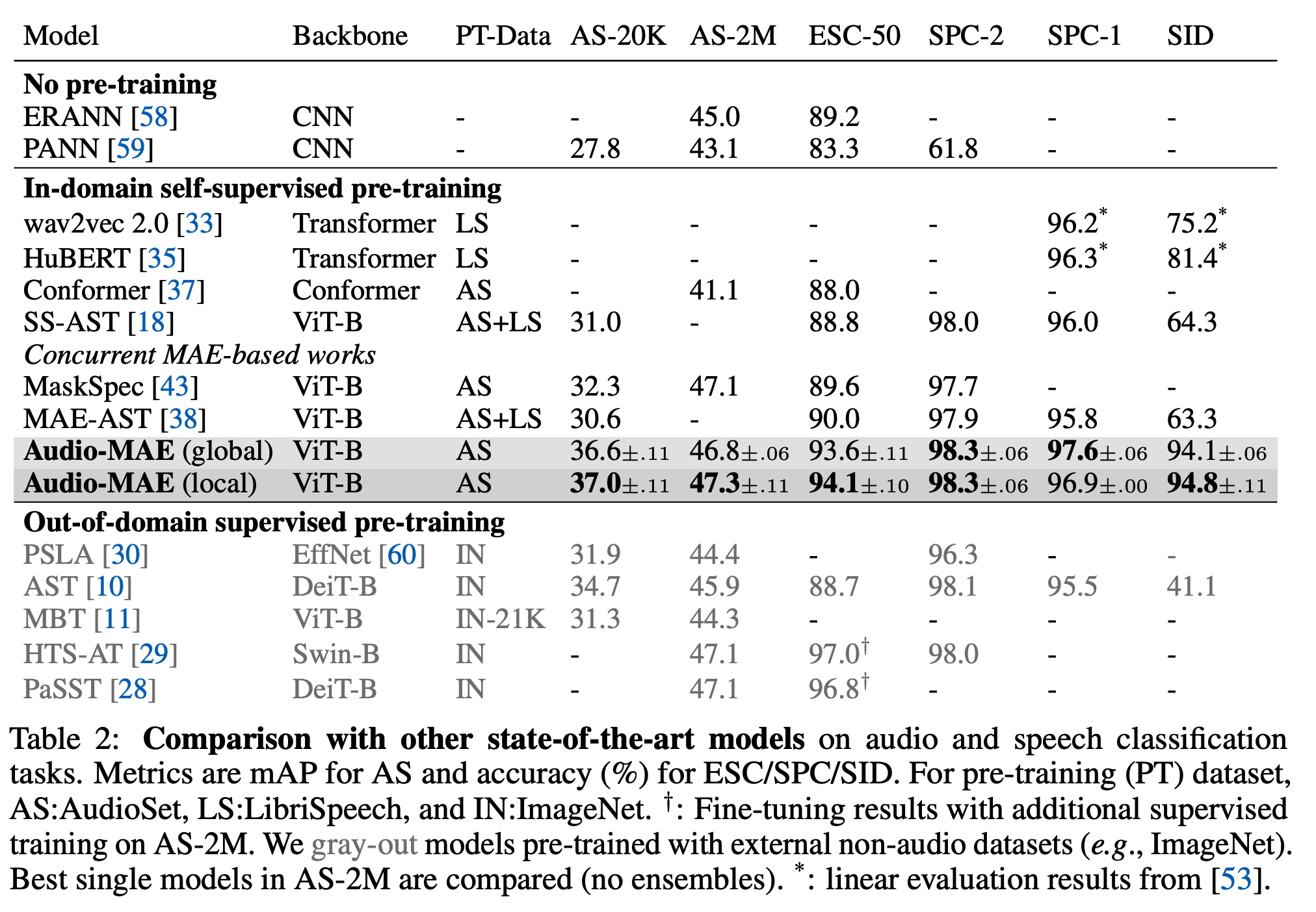
Comparison into 3 groups

• For fair comparison, our main benchmark is the (1) models using SSL pre-training on in-domain (audio) datasets (AudioSet and LibriSpeech).

• (2) without pre-training & (3) supervised pre-training on out-of-domain ImageNet

Summary: with audio-only from-scratch pre-training on AudioSet, Audio-MAE performs well for both the audio and speech classification tasks.

(6) Visualization