71.DropMax, Adaptive Variational Softmax

DropMax : Adaptive Variational Softmax (NeurIPS 2018)

Abstract

DropMax : stochastic version of softmax classifier

• at each iteration, drops non-target classes, according to dropout probabilities

• binary masking over class output probabilities

  ( input-adaptively learned via VI )

• stochastic regularization

  \(\rightarrow\) has an effect of building ensemble classifier with different decision boundaries

1. Introduction

propose a novel variant of softmax classifier

• improved accuracy over regular softmax

• at each stochastic gradient descent :

  • applies dropout to the exponentiations in the softmax

• allows the classifier to be learned to solve a distinct subproblem

  ( enabling focus on discriminative properties )

• ensemble classifier with different decision boundaries

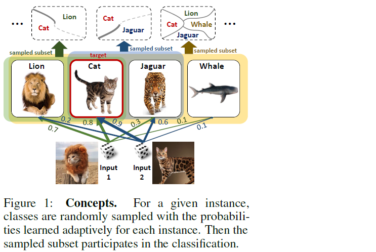
Extend the classifier to LEARN the probability of dropping non-target class!

can be viewed as stochastic attention mechanism

• selects a subset of classes each instance should attend to!

Contribution

• 1) DropMax that randomly drops non-target classes
• 2) propose VI framework to adaptively learn the dropout probability of non-target class
• 3) incorporate label info into our conditional VI

2. Related Work

(1) Subset sampling with softmax classifier

Existing works :

• consider only a “partial subset of classes” to improve efficiency

  ex) negative sampling

(2) Dropout Variational Inference

Bayesian understanding of Dropout(DO)

• DO can also be understood as noise injection process
• network trained with DO can be seen as deep GP

(3) Learnisng dropout probability

Generally, d.o rate is “tunable parameter”, not something “learned”

Recent proposed models allow to learn d.o rate

• Variational Dropout
  • each weight has independent Gaussian with mean&var that are trained with reparam trick
  • due to CLT, Gaussian dropout is identical to binary dropout, with faster convergence

3. Approach

Notation

• \(\mathcal{D}=\left\{\left(\mathbf{x}_{i}, \mathbf{y}_{i}\right)\right\}_{i=1}^{N}\) : dataset
  • \(\mathbf{x}_{i} \in \mathbb{R}^{d}\), \(\mathbf{y}_{i} \in\{0,1\}^{K}\)
  • \(K\) : number of classes
• \(\mathbf{h}=\mathrm{NN}(\mathrm{x} ; \omega),\) : last feature vector generated by NN, parameterized by \(w\)

K-dimensional class logits ( or scores ) :

• \(\mathbf{o}(\mathbf{x} ; \psi)=\mathbf{W}^{\top} \mathbf{h}+\mathbf{b}, \quad \psi=\{\mathbf{W}, \mathbf{b}\}\).

Softmax Classifier :

• \(p(\mathbf{y} \mid \mathbf{x} ; \psi)=\frac{\exp \left(o_{t}(\mathbf{x} ; \psi)\right)}{\sum_{k} \exp \left(o_{k}(\mathbf{x} ; \psi)\right)}\).

3-1. DropMax

Propose to randomly drop out classes at training phase

when \(\exp(o_k)=0\), then class \(k\) is excluded from the classification & gradients are not back-propagated

Randomly drop \(\exp(o_1)=0,...,\exp(o_k)=0\), based on Bernoulli trials

• by introducing dropout binary mask vector \(z_k\)
• retain probability \(\rho_k\)

\[z_{k} \sim \operatorname{Ber}\left(z_{k} ; \rho_{k}\right), \quad p(\mathbf{y} \mid \mathbf{x}, \mathbf{z} ; \psi)=\frac{\left(z_{t}+\varepsilon\right) \exp \left(o_{t}(\mathbf{x} ; \psi)\right)}{\sum_{k}\left(z_{k}+\varepsilon\right) \exp \left(o_{k}(\mathbf{x} ; \psi)\right)}\]

However, if we drop classes based on purely random Bernoulli trials,

we may exclude classes that are important for classification

\(\rightarrow\) adopt the idea of Adaptive Dropout , and model \(\rho\) as an output of NN

• \(\rho(\mathrm{x} ; \theta)=\operatorname{sgm}\left(\mathbf{W}_{\theta}^{\top} \mathbf{h}+\mathbf{b}_{\theta}\right), \quad \theta=\left\{\mathbf{W}_{\theta}, \mathbf{b}_{\theta}\right\}\). ( have to learn param \(\theta\) )

• \(z_{k} \mid \mathbf{x} \sim \operatorname{Ber}\left(z_{k} ; \rho_{k}(\mathbf{x} ; \theta)\right), \quad p(\mathbf{y} \mid \mathbf{x}, \mathbf{z} ; \psi, \theta)=\frac{\left(z_{t}+\varepsilon\right) \exp \left(o_{t}(\mathbf{x} ; \psi)\right)}{\sum_{k}\left(z_{k}+\varepsilon\right) \exp \left(o_{k}(\mathbf{x} ; \psi)\right)}\).

Difference with Adaptive Dropout?

• (Adaptive Dropout) drop “neurons”
• (Dropmax) drop “classes”

Limitation : high variance during training….

• thus use concrete distribution

  ( = continuous relaxation of discrete r.v , that allows to back-propagate through the \(z_k\))

• \(z_{k}=\operatorname{sgm}\left\{\tau^{-1}\left(\log \rho_{k}(\mathbf{x} ; \theta)-\log \left(1-\rho_{k}(\mathbf{x} ; \theta)\right)+\log u-\log (1-u)\right)\right\}\).

  with \(u \sim Unif(0,1)\)

4. Approximate Inference for Dropmax

Learning framework for DropMaxx

4-1. Intractable True posterior

\[p(\mathbf{Z} \mid \mathbf{X}, \mathbf{Y})=\prod_{i=1}^{N} p\left(\mathbf{z}_{i} \mid \mathbf{x}_{i}, \mathbf{y}_{i}\right)\]

Mean field assumption : \(p(\mathbf{z} \mid \mathbf{x})=\prod_{k=1}^{K} p\left(z_{k} \mid \mathbf{x}\right)\)

• but unlike \(p(\mathbf{z} \mid \mathbf{x})\), \(p(\mathbf{z} \mid \mathbf{x},\mathbf{y})\) is not decomposable into the product of each element

\(\rightarrow\) use SGVB (Stochastic Gradient Variational Bayes)

​ ( approximating intractable posterior of latent variables in NN )

maximize ELBO :

\(\log p(\mathbf{Y} \mid \mathbf{X} ; \psi, \theta) \geq \sum_{i=1}^{N}\left\{\mathbb{E}_{q\left(\mathbf{z}_{i} \mid \mathbf{x}_{i}, \mathbf{y}_{i} ; \phi\right)}\left[\log p\left(\mathbf{y}_{i} \mid \mathbf{z}_{i}, \mathbf{x}_{i} ; \psi\right)\right]-\mathrm{KL}\left[q\left(\mathbf{z}_{i} \mid \mathbf{x}_{i}, \mathbf{y}_{i} ; \phi\right) \mid \mid p\left(\mathbf{z}_{i} \mid \mathbf{x}_{i} ; \theta\right)\right]\right\}\).

4-2. Structural form of the approximate posterior

How to encode using NN?

(1) encode the structural form of the true posterior ( can be decomposed as below )

• \(p(\mathbf{z} \mid \mathbf{x}, \mathbf{y})=\underbrace{p(\mathbf{z} \mid \mathbf{x})}_{\mathcal{A}} \times \underbrace{p(\mathbf{y} \mid \mathbf{z}, \mathbf{x}) / p(\mathbf{y} \mid \mathbf{x})}_{\mathcal{B}}\).
  • \(\mathcal{B}\) : rescaling factor
  • \(\mathcal{A} = p(\mathbf{z} \mid \mathbf{x} ; \theta)=\operatorname{Ber}\left(\mathbf{z} ; \operatorname{sgm}\left(\mathbf{W}_{\theta}^{\top} \mathbf{h}+\mathbf{b}_{\theta}\right)\right)\).
  • to make \(\mathcal{B}\), just add \(\mathrm{r} \in \mathbb{R}^{K}\) to the \(\mathcal{A}\) & squash it to range \([0,1]\)

\(\mathbf{g}(\mathbf{x} ; \phi)=\operatorname{sgm}\left(\overline{\mathbf{W}}_{\theta}^{\top} \mathbf{h}+\overline{\mathbf{b}}_{\theta}+\mathbf{r}(\mathbf{x} ; \phi)\right), \quad \mathbf{r}(\mathbf{x} ; \phi)=\mathbf{W}_{\phi}^{\top} \mathbf{h}+\mathbf{b}_{\phi}\).

• \(\phi=\left\{\mathbf{W}_{\phi}, \mathbf{b}_{\phi}\right\}\) is variational parameter

4-3. Encoding the label information

modeling choice for encoding \(y\) is based on…

Observation 1

each \(r_{t}(\mathrm{x} ; \phi)\) and \(r_{k \neq t}(\mathrm{x} ; \phi)\) should be maximized and minimized respectively…

by minimizing cross-entropy :

\(\mathcal{L}_{\text {aux }}(\phi)=-\sum_{i=1}^{N} \sum_{k=1}^{K}\left\{y_{i, k} \log \operatorname{sgm}\left(r_{k}\left(\mathrm{x}_{i} ; \phi\right)\right)+\left(1-y_{i, k}\right) \log \left(1-\operatorname{sgm}\left(r_{k}\left(\mathrm{x}_{i} ; \phi\right)\right)\right)\right\}\)>

Observation 2

\(\mathbf{z}_{\backslash t} \neq \mathbf{0} \rightarrow z_{t}=1\) given \(\mathbf{y}\).

ignoring the case \(\mathbf{z}_{\backslash t}=\mathbf{0}\) and fixing \(q\left(z_{t} \mid \mathbf{x}, \mathbf{y} ; \phi\right)=\operatorname{Ber}\left(z_{t} ; 1\right)\) is a close approximation of \(p\left(z_{t} \mid \mathbf{x}, \mathbf{y}\right)\)

Thus, final approximate posterior is :

\(q(\mathbf{z} \mid \mathbf{x}, \mathbf{y} ; \phi)=\operatorname{Ber}\left(z_{t} ; 1\right) \prod_{k \neq t} \operatorname{Ber}\left(z_{k} ; g_{k}(\mathbf{x} ; \phi)\right)\).

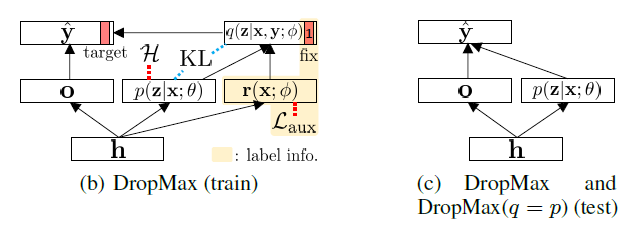
4.4 Regularized variational inference

critical issue in optimizing ELBO :

= \(p(\mathbf{z} \mid \mathbf{x} ; \theta)\) collapses into \(q(\mathbf{z} \mid \mathbf{x}, \mathbf{y} ; \phi)\) too easily!

• crucial for \(\mathbf{z}\) to generalize well on test instance

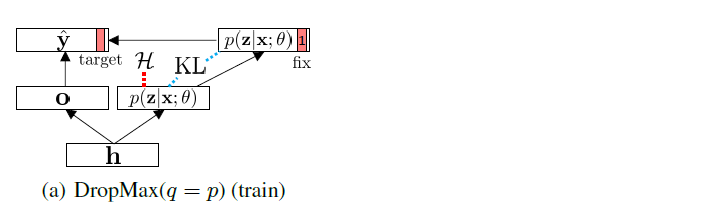
Instead of weight-decay, use “entropy regularizer” directly to \(p(\mathbf{z} \mid \mathbf{x} ; \theta)\)

• \(\mathcal{H}(p(\mathbf{z} \mid \mathbf{x} ; \theta))=\sum_{k} \rho_{k} \log \rho_{k}+\left(1-\rho_{k}\right) \log \left(1-\rho_{k}\right)\).

KL divergence & final minimization objective :

\(\begin{array}{l} \mathrm{KL}[q(\mathbf{z} \mid \mathbf{x}, \mathbf{y} ; \phi) \mid \mid p(\mathbf{z} \mid \mathbf{x} ; \theta)]=\sum_{k}\left\{\mathbb{I}_{\{k=t\}} \log \frac{1}{\rho_{k}}+\mathbb{I}_{\{k \neq t\}}\left(g_{k} \log \frac{g_{k}}{\rho_{k}}+\left(1-g_{k}\right) \log \frac{1-g_{k}}{1-\rho_{k}}\right)\right\} \\ \mathcal{L}(\psi, \theta, \phi)=\sum_{i=1}^{N}\left[-\frac{1}{S} \sum_{s=1}^{S} \log p\left(y_{i} \mid \mathbf{x}_{i}, \mathbf{z}_{i}^{(s)} ; \psi\right)+\operatorname{KL}\left[q\left(\mathbf{z}_{i} \mid \mathbf{x}_{i}, \mathbf{y}_{i} ; \phi\right) \mid \mid p\left(\mathbf{z}_{i} \mid \mathbf{x}_{i} ; \theta\right)\right]-\mathcal{H}\right]+\mathcal{L}_{\mathrm{aux}} \end{array}\).

Testing

Monte-Carlo sampling : \(p\left(\mathbf{y}^{*} \mid \mathbf{x}^{*}\right)=\mathbb{E}_{\mathbf{z}}\left[p\left(\mathbf{y}^{*} \mid \mathbf{x}^{*}, \mathbf{z}\right)\right] \approx \frac{1}{S} \sum_{s=1}^{S} p\left(\mathbf{y}^{*} \mid \mathbf{x}^{*}, \mathbf{z}^{(s)}\right), \quad \mathbf{z}^{(s)} \sim p\left(\mathbf{z} \mid \mathbf{x}^{*} ; \theta\right)\).

Approximate : \(p\left(\mathbf{y}^{*} \mid \mathbf{x}^{*}\right)=\mathbb{E}_{\mathbf{z}}\left[p\left(\mathbf{y}^{*} \mid \mathbf{x}^{*}, \mathbf{z}\right)\right] \approx p\left(\mathbf{y}^{*} \mid \mathbf{x}^{*}, \mathbb{E}\left[\mathbf{z} \mid \mathbf{x}^{*}\right]\right)=p\left(\mathbf{y}^{*} \mid \mathbf{x}^{*}, \rho\left(\mathbf{x}^{*} ; \theta\right)\right)\).

5. Conclusion

stochastic version of a softmax function, DropMax

• enable to build ensemble over exponentially many classifiers

cast this as Bayesian learning problem

• present how to optimize params through VI
• propose novel regularizer