70.Bayesian Adversarial Learning

Bayesian Adversarial Learning (NeurIPS 2018)

Abstract

DNN : vulnerable to adversarial attacks

\(\rightarrow\) popular defense : “robust optimization problem”

( = minimizes a “point estimate” of worst-case loss )

BUT, point estimate ignores potential test adversaries that are beyond pre-defined constraints

This paper proposes Bayesian Robust Learning

• “distribution” ( instead of point estimate ) is put on the adversarial data-generating distribution to account for the uncertainty of the adversarial data-generating process

1. Introduction

DL : vulnerable to maliciously manipulated & imperceptible perturbation over original data

• ex) “ADVERSARIAL EXAMPLES”
• security-sensitive scenarios!

Adversarial training

• generated adversarial examples are fet to NN as augmented data, to enhance robustness

Distributionally robust optimization problem

• idea : ‘minimize the worst-case loss’ w.r.t perturbed data distribution

Most existing robust learning approaches solve a “point estimate” of either

• worst-case per-datum perturbation
• adversary data-generating distribution

Novel Framework for robust learning, BAYESIAN ADVERSARIAL LEARNING (BAL)

2. Bayesian Adversarial Learning

2 players : (1) data generator & (2) learner

(1) data generator

• modify training data \(D\) into perturbed on \(\tilde{D}\)
• fool the learner’s prediction

(2) learner

• tries to predict best on the \(\tilde{D}\)

Introduce fully Bayesian treatment of both (1) & (2)

• put an energy-based pdf over \(\tilde{D}\)

  ( = distribution over data distribution, to quantify “uncertainty” of data generating process )

• \(p(\tilde{\mathcal{D}} \mid \boldsymbol{\theta}, \mathcal{D}) \propto \exp \{L(\tilde{\mathcal{D}} ; \boldsymbol{\theta})-\alpha c(\tilde{\mathcal{D}}, \mathcal{D})\}\).

  • loss function \(L(\tilde{\mathcal{D}} ; \boldsymbol{\theta})\) : predicting on the perturbed data \(\tilde{\mathcal{D}}\) given the learner’s strategy \(\boldsymbol{\theta}\)
    • high loss \(\rightarrow\) high energy
  • cost \(c(\tilde{\mathcal{D}}, \mathcal{D})\) : cost of modifying \(D\) to \(\tilde{D}\)
    • high cost \(\rightarrow\) low energy
  • \(\alpha\) : hyperparameter

Learner samples its model parameter \(\theta\)

• \(p(\boldsymbol{\theta} \mid \tilde{\mathcal{D}}) \propto \exp \{-L(\tilde{\mathcal{D}} ; \boldsymbol{\theta})\} p(\boldsymbol{\theta} \mid \beta)\).

  • \(p(\boldsymbol{\theta} \mid \beta)\): prior

  • \(\beta\) : hyperparameter

by BAL, obtain robust posterior over learner’s parameter \(\theta\)

( by Gibbs sampling )

• \(p(\tilde{\mathcal{D}} \mid \boldsymbol{\theta}, \mathcal{D}) \propto \exp \{L(\tilde{\mathcal{D}} ; \boldsymbol{\theta})-\alpha c(\tilde{\mathcal{D}}, \mathcal{D})\}\).

  \(p(\boldsymbol{\theta} \mid \tilde{\mathcal{D}}) \propto \exp \{-L(\tilde{\mathcal{D}} ; \boldsymbol{\theta})\} p(\boldsymbol{\theta} \mid \beta)\).

• at \(i^{th}\) iteration…

  • \(\tilde{\mathcal{D}}^{(t)} \mid \boldsymbol{\theta}^{(t-1)}, \mathcal{D} \sim p\left(\tilde{\mathcal{D}} \mid \boldsymbol{\theta}^{(t-1)}, \mathcal{D}\right)\).
  • \(\boldsymbol{\theta}^{(t)} \mid \tilde{\mathcal{D}}^{(t)} \sim p\left(\boldsymbol{\theta} \mid \tilde{\mathcal{D}}^{(t)}\right)\).

• after burn-in period, collected sample \(\left\{\boldsymbol{\theta}^{(T)}, \tilde{\mathcal{D}}^{(T)}\right\}\) follows the “joint posterior” \(p(\boldsymbol{\theta}, \tilde{\mathcal{D}} \mid \mathcal{D})\).

  ( different from existing approaches using “point estimate” )

• TEST time : prediction w.r.t the posterior

  \(p\left(y_{*} \mid \mathbf{x}_{*}, \mathcal{D}\right)=\int p\left(y_{*} \mid \mathbf{x}_{*}, \boldsymbol{\theta}\right) p(\boldsymbol{\theta} \mid \mathcal{D}) d \boldsymbol{\theta} \approx \frac{1}{T} \sum_{t=1}^{T} p\left(y_{*} \mid \mathbf{x}_{*}, \boldsymbol{\theta}^{(t)}\right), \quad \boldsymbol{\theta}^{(t)} \sim p(\boldsymbol{\theta} \mid \mathcal{D})\).

To make BAL framework practical… have to specify

• 1) how to generate \(\tilde{D}\) based on \(D\)
• 2) configuration of the cost function \(c(\tilde{D},D)\)
• 3) learner’s model family \(f(\mathbf{x} ; \theta)\) and \(p(y \mid f(\mathbf{x} ; \theta))\)

3. A Practical Instantiation of BAL

3-1. Data Generator

Data generator :

• only modifies input
• \(p(\tilde{\mathcal{D}} \mid \boldsymbol{\theta}, \mathcal{D})=p(\tilde{\mathbf{X}} \mid \boldsymbol{\theta}, \mathbf{X})=\prod_{i=1}^{N} p\left(\tilde{\mathbf{x}}_{i} \mid \boldsymbol{\theta}, \mathbf{x}_{i}\right) \propto \exp \left\{\sum_{i=1}^{N} \ell\left(\tilde{\mathbf{x}}_{i} ; \boldsymbol{\theta}\right)-\alpha \sum_{i=1} c\left(\tilde{\mathbf{x}}_{i}, \mathbf{x}_{i}\right)\right\}\)… eq (A)
  • loss function \(L(\cdot)\)
    • negative log likelihood …. \(\ell(\tilde{\mathbf{x}} ; \boldsymbol{\theta})=-\log p(y \mid f(\tilde{\mathbf{x}} ; \boldsymbol{\theta}))\)
  • cost function
    • L2 distance … \(c(\tilde{\mathbf{x}}, \mathbf{x})= \mid \mid \tilde{\mathbf{x}}-\mathbf{x} \mid \mid _{2}^{2}\)

Key difference from existing robust optimization method :

• instead of finding a single worst-case perturbed data,

  probability distribution is put over the generated data distn

• thus, can fully capture all possible cases of generated data

  \(\rightarrow\) enhance learner’s robustness

3-2. Learner

given generated \(\tilde{X}\), leaner provides optimal \(\theta\) by sampling from below conditional distn :

• \(p(\boldsymbol{\theta} \mid \tilde{\mathbf{X}}) \propto \exp \left\{-\sum_{i=1}^{N} \ell\left(\tilde{\mathbf{x}}_{i} ; \boldsymbol{\theta}\right)\right\} p(\boldsymbol{\theta} \mid \beta)\)… eq (B)

3-3. Iterative Gibbs sampling

eq (A) & eq (B)

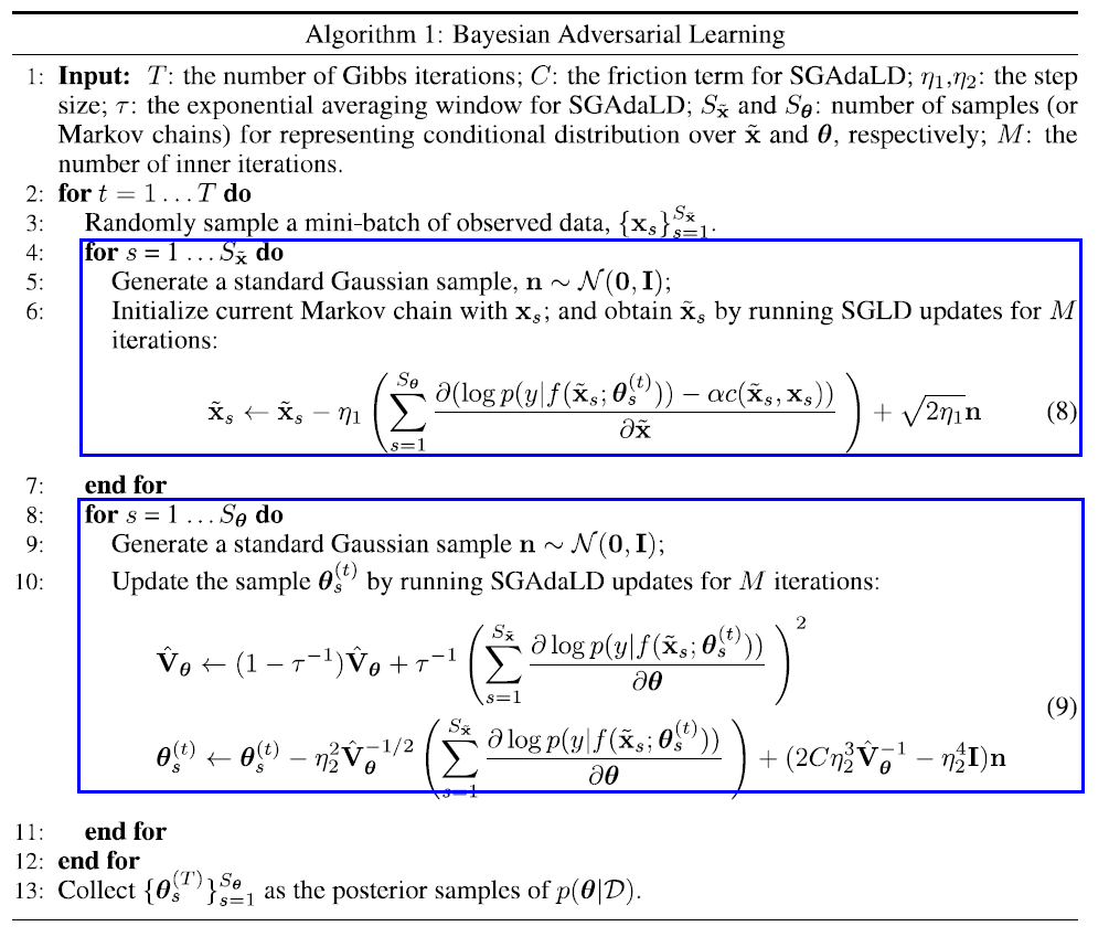
4. Algorithm

4-1. Scalable Sampling

(a) when sampling fake data

sampling full data from \(p(\tilde{\mathbf{X}} \mid \boldsymbol{\theta}, \mathbf{X})\) is expensive

\(\rightarrow\) thus resort to stochastic optimization

• sample mini-batch \(\{\tilde{\mathbf{x}}\}_{s=1}^{S_{\tilde{\mathbf{x}}}}\)
• use SGLD ( Stochastic Gradient Langevin Dynamics ) to achieve scalable sampling

(b) when sampling the posterior of model params

naive SGHMC sampler cannot efficiently explore the target density, due to high correlation

\(\rightarrow\) use

• for simplicity, do not use momentum term \(\rightarrow\) SGAdaLD
• \(\boldsymbol{\theta} \leftarrow \boldsymbol{\theta}-\eta^{2} \hat{\mathbf{V}}_{\boldsymbol{\theta}}^{-1 / 2} \mathbf{g}_{\boldsymbol{\theta}}+\mathcal{N}\left(0,2 C \eta^{3} \hat{\mathbf{V}}_{\boldsymbol{\theta}}^{-1}-\eta^{4} \mathbf{I}\right)\).

4-2. Connection to other defensive methods

characteristics of BAL by comparing with otehrs

• 1) fully Bayesian Approach
• 2) BNN also constructs posterior distn over \(\theta\), but BAL yields stronger robustness
• 3) Bayesian GAN : proposed for generative modeling, not adversarial learning

5. Conclusion

proposed adversarial training method, Bayesian Adversarial Learning(BAL)

• scalable sampling strategy
• practical safety-critical problem