
Divide And Couple : Using Monte Carlo Variational Objectives for Posterior ( NeurIPS 2019 )
Abstract
recent VI : use idea from MC estimation to make tighter bounds
given a VI objective (defined by MC estimator of likelihood)….use Divide and Couple
- to identify augmented proposal & target distn
- so that the gap between
- “VI objective” & “log-likelihood” is equal to
- the divergence between “augmented proposal” & “target distn”
1. Introduction
VI : \(\log p(x)=\underset{q(\mathbf{z})}{\mathbb{E}}\left[\log \frac{p(\mathbf{z}, x)}{q(\mathbf{z})}\right]+\mathrm{KL}[q(\mathbf{z}) \mid \mid p(\mathbf{z} \mid x)]\).
Tighter objectives :
- let \(R\) be the estimator of likelihood
- \(\mathbb{E} R=\) \(p(x)\) .
- \(\log p(x) \geq \mathbb{E} \log R\) ( by Jensen’s Inequality )
- Standard \(\mathrm{VI}\) : \(R=p(z, x) / q(z)\)
- Importance-weighted autoencoders (IWAEs) : \(R=\frac{1}{M} \sum_{m=1}^{M} p\left(\mathbf{z}_{m}, x\right) / q\left(\mathbf{z}_{m}\right)\)
show how to find a distn \(Q(z)\) such that
- divergence between \(Q(z)\) and \(p(z \mid x)\) is at most the gap between \(\mathbb{E} \log R\) and \(\log p(x)\).
- Thus, “better estimator” = “better posterior approximations”
- how to find \(Q(z)\) ? by divide and couple
Divide and Couple
- Divide : maximize \(\mathbb{E} \log R\) = minimize gap between \(\mathbb{E} \log R\) and \(\log p(x)\).
- Couple : divergence is an upper bound to \(\mathrm{KL}[Q(\mathrm{z}) \mid \mid p(\mathrm{z} \mid x)]\).
2. Setup and Motivation
ELBO decomposition & Jensen’s Inequality
- \(\log p(x) \geq \mathbb{E} \log R\).
- traditional VI ) \(R=p(\mathrm{z}, x) / q(\mathrm{z})\)
- Many other estimators \(R\) of \(p(x)\)….
2-1. Example
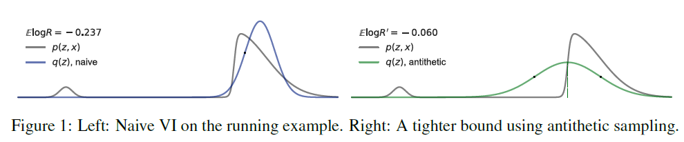
Target distn \(p(z,x)\) & Gaussian \(q(z)\)
Tightening the likelihood bound has made \(q\) cloes to \(p\)
**Antithetic sampling **
-
\(R^{\prime}=\frac{1}{2}\left(\frac{p(z, x)+p(T(z), x)}{q(z)}\right), z \sim q\).
where \(T(z) = \mu - (z - \mu)\).
- \(z\) “reflected” around the mean \(\mu\) of \(q\)
3. The Divide-and-Couple Framework
Posterior inference for general non-negative estimators, using divide & couple
3-1. Divide
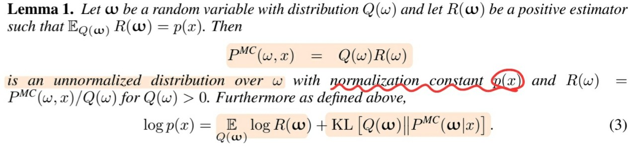
\(\mathbb{E}_{Q(\boldsymbol{\omega})} R(\boldsymbol{\omega})=p(x)\), where \(\boldsymbol{\omega} \sim Q(\omega)\).
Divide step
-
interpret \(\mathbb{E}_{Q(\boldsymbol{\omega})} R(\boldsymbol{\omega})\) as an ELBO, by defining \(P^{MC}\)
so that \(R(\omega)=P^{\mathrm{MC}}(\omega, x) / Q(\omega)\).
-
\(P^{MC}\) and \(Q\) divide to produce \(R\)
3-2. Couple
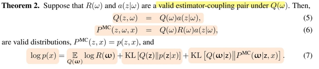
Suggest coupling \(P^{\mathrm{MC}}(\omega, x)\) and \(p(z, x)\)
into some new distribution (augmented distribution) \(P^{\mathrm{MC}}(\omega, z, x)\) with \(P^{\mathrm{MC}}(z, x)=p(z, x) .\)
for \(P^{\mathrm{MC}}(z, \omega, x)=\) \(P^{\mathrm{MC}}(\omega, x) a(z \mid \omega)\) to be a valid coupling,
we require that \(\int P^{\mathrm{MC}}(\omega, x) a(z \mid \omega) d \omega=p(z, x)\).
- Key Point : if \(R\) is a good estimator, it means that…
- \(\mathbb{E} \log R\) is close to \(\log p(x)\)
- \(Q(z)\) must e close to \(p(z \mid x)\)
3-3. Example
\(R^{\prime}=\frac{1}{2}\left(\frac{p(z, x)+p(T(z), x)}{q(z)}\right), z \sim q\).
- tighter VI
- but less similar to the target! ( check the figure below )
Since \(Q(w)\) is a poor approximation.. how can we solve?
consider coupling distn
-
\(a(z \mid \omega)=\pi(\omega) \delta(z-\omega)+(1-\pi(\omega)) \delta(z-T(\omega))\).
-
\(\pi(\omega)=\frac{p(\omega, x)}{p(\omega, x)+p(T(\omega), x)}\).
Thus, the augmented variational distn is \(Q(\omega, z)=Q(\omega) a(z \mid \omega)\).
- draw \(\omega \sim Q\) and select \(z=\omega\) with probability \(\pi(\omega)\) or \(z=T(\omega)\) otherwis
4. Conclusion
Central Insight :
-
approximate posterior can be constructed from an estimator using “coupling”
( this posterior’s divergence is bounded by the looseness of the likelihood bound )