84.Averaging Weights Leads to Wider Optima and Better Generalization

Averaging Weights Leads to Wider Optima and Better Generalization (2018)

Abstract

DNN : trained by optimizing loss function with an SGD variant

Show that simple averaging of multiple points along the trajectory of SGD, with cyclical or constant learning rate, leads to better generalization.

Propose SWA (Stochastic Weight Averaging)

1. Introduction

better understanding of the loss surface \(\rightarrow\) accelerate convergence

local optima found by SGD can be connected by simple curves!

• Fast Geometric Ensembling (FGE) : sample multiple nearby points in “the weight space”

• propose Stochastic Weight Averaging (SWA)

Contribution

• SGD with cyclical & constant learning rates traverses regions of weight space corresponding to high-performance networks
• FGE ensembles :
  • can be trained in the same time as a single model
  • test predictions for an ensemble of \(k\) models requires \(k\) times more computation
• SWA leads to solutions that are wider than the optima found by SGD

2. Related Work

Better understanding of geometry of loss surfaces & generaliztion in DL

SWA is related to work in both (1) optimization & (2) regularization

• SGD is more likely to converge to broad local optima than batch gradient
  • more likely tho have good test performance
• SWA is based on averaging multiple points
• to enforce exploration, run SGD with “constant or cyclical learning rates”

FGE (Fast Geometric Ensembling)

• using a cyclical learning rate, it is possible to gather models that are spatially close to each other, but produce diverse predictions

Dropout

• approach to regularize DNNs
• different architecture is created
• dropout = ensemble = Bayesian model averaging

3. Stochastic Weight Averaging

Section 3-1 : trajectories of SGD with a constant and cyclical learning rate

Section 3-2 : SWA algorithm

Section 3-3 : complexity

Section 3-4 : widths of solutions ( SWA vs SGD )

SWA has 2 meanings

• 1) it is an average of SGD weights
• 2) approximately sampling from the loss surface of the DNN, leading to stochastic weights

3-1. Analysis of SGD Trajectories

Cyclical learning rate schedule

• linearly decrease the learning rate from \(\alpha_1\) to \(\alpha_2\)

  \(\begin{array}{l} \alpha(i)=(1-t(i)) \alpha_{1}+t(i) \alpha_{2} \\ t(i)=\frac{1}{c}(\bmod (i-1, c)+1) \end{array}\).

For even greater exploration, we consider “constant learning rate” \(\alpha(i)=\alpha_1\)

Both methods are doing exploration in the region of space corresponding to DNNs with high accuracy.

Main Difference :

individual proposals of SGD with cyclical learning rate schedule > ~ fixed rate schedule

• (cyclical) spends several epochs fine tuning, after large steps
• (fixed) always making steps of relatively large sizes ( explore more efficiently )

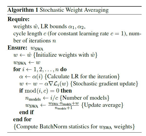
3-2. SWA Algorithm

(1) start with a pretrained model \(\hat{w}\)

• can be trained with conventional training procedure

(2) stop the training early

• without modifying the lr schedule

(3) starting from \(\hat{w}\), continue training

• using cyclical or constant lr schedule

SWA is related to FGE, except …

• FGE : averaging the predictions of the models
• SWA : average their weights

3-3. Computational Complexity

During Training

• need to maintain a copy of the running average of DNN weights

After Training

• only need to store the model that aggergates the average

  ( = same memory requirements as standard training )

Extra time : only spent to update the aggregated weight average :

• \(w_{\mathrm{SWA}} \leftarrow \frac{w_{\mathrm{SWA}} \cdot n_{\mathrm{models}}+w}{n_{\mathrm{models}}+1}\).

3-4. Solution Width

Width of a local optimum is related to generalization

\(\begin{array}{l} w_{\mathrm{SWA}}(t, d)=w_{\mathrm{SWA}}+t \cdot d \\ w_{\mathrm{SGD}}(t, d)=w_{\mathrm{SGD}}+t \cdot d \end{array}\).

Line Segment connecting those two

• \(w(t)=t \cdot w_{\mathrm{SGD}}+(1-t) \cdot w_{\mathrm{SWA}}\).

3-5. Connection to Ensembling

FGE (Fast Geometric Ensembling)

• training ensembles in the time required to train a single model

• using cyclical l.r, generates a sequence of points

  that are close in weight space, but produce different predictions

SWA

• instead of averaging the predictions, average their weights

Similarities between FGE & SWA

FGE

• \(\bar{f}=\frac{1}{n} \sum_{i=1}^{n} f\left(w_{i}\right)\).

SWA

• average \(w_{\text {SWA }}=\frac{1}{n} \sum_{i=1}^{n} w_{i}\).
• \(\Delta_{i}=w_{i}-w_{\mathrm{SWA}}\).
• linearization of \(f\) at \(w_{SWA}\) : \(f\left(w_{j}\right)=f\left(w_{\mathrm{SWA}}\right)+\left\langle\nabla f\left(w_{\mathrm{SWA}}\right), \Delta_{j}\right\rangle+O\left( \mid \mid \Delta_{j} \mid \mid ^{2}\right)\)

Difference between averaging the weights & averaging the predictions

\(\begin{array}{c} \bar{f}-f\left(w_{\mathrm{SWA}}\right)=\frac{1}{n} \sum_{i=1}^{n}\left(\left\langle\nabla f\left(w_{\mathrm{SWA}}\right), \Delta_{i}\right\rangle+O\left( \mid \mid \Delta_{i} \mid \mid ^{2}\right)\right) \\ =\left\langle\nabla f\left(w_{\mathrm{SWA}}\right), \frac{1}{n} \sum_{i=1}^{n} \Delta_{i}\right\rangle+O\left(\Delta^{2}\right)=O\left(\Delta^{2}\right), \end{array}\).

Difference between the predictions of different perturbed networks :

• \(f\left(w_{i}\right)-f\left(w_{j}\right)=\left\langle\nabla f\left(w_{\mathrm{SWA}}\right), \Delta_{i}-\Delta_{j}\right\rangle+O\left(\Delta^{2}\right)\).

conclusion : SWA can approximate the FGE ensemble with a single model!