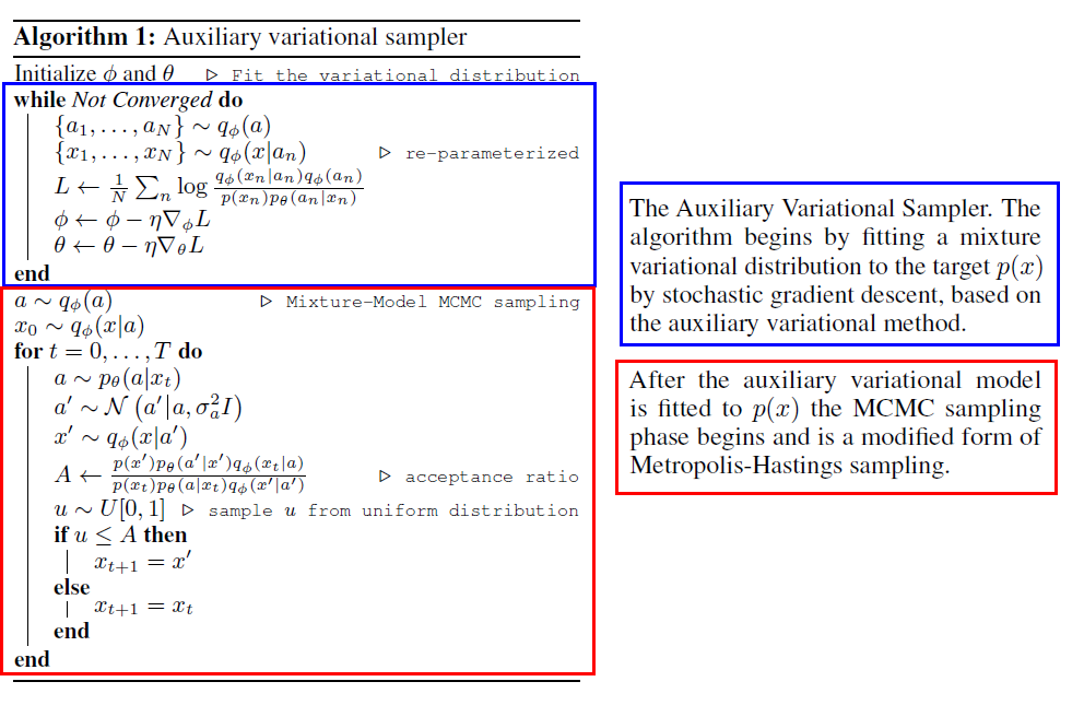
Auxiliary Variational MCMC
Abstract
Auxiliary Variational MCMC = (1) + (2)
- (1) MCMC kernels
- (2) Variational Inference
Exploits LOW dimensional structure in the target distribution,
in order to learn a MORE EFFICIENT MCMC sampler
1. Introduction
Naive pairing of (1) & (2) :
- use “variational approximation \(q\)” as a “proposal distribution” in a M-H sampler
This paper suggests alternative approach, inspired by..
- 1) BBVI (Black-Box Variational Inference)
- 2) auxiliary variable MCMC ( ex. HMC )
Contribution
- 1) general framework for VI + MCMC
- 2) use auxiliary variational method to capture latent low-dim structure in target distn
- 3) extension of M-H algorithm to continuous mixture proposals
- 4) introduce Auxiliary Variational Sampler (AVS)
- use flexible distns, parameterized by NN
2. Auxiliary Variational MCMC
Key idea : exploit structure present in the target distn \(p(x)\)
-
by fitting parameterized variational approximation in the AUGMENTED space
\(\rightarrow\) allows to learn “low-dimensional” structure
Introduce auxiliary variable method & how to combine with proposal distns
2-1. Mixture Proposal MCMC
Notation :
- \(\tilde{q}\) : proposal distn
- \(q\) : variational distn
for valid MCMC, need ERGODIC Markov chain, whose stationary distn = \(p(x)\) ( target distn )
\(\rightarrow\) introduce M-H like algorithm, with a specially chosen form of proposal distn
( This proposal can be combined with auxiliary variational method !)
(1) Mixture proposal distribution
-
\(\tilde{q}\left(x^{\prime} \mid x\right)=\int \tilde{q}\left(x^{\prime} \mid a\right) \tilde{q}(a \mid x) d a\).
-
sampling step )
-
Sample \(a\) from \(\tilde{q}(a \mid x)\)
-
Sample \(x^{\prime}\) from \(\tilde{q}\left(x^{\prime} \mid a\right)\)
-
Accept the candidate sample \(x^{\prime}\) with probability
\(\min \left\{1, \frac{\tilde{q}(x \mid a) \tilde{q}\left(a \mid x^{\prime}\right) p\left(x^{\prime}\right)}{\tilde{q}\left(x^{\prime} \mid a\right) \tilde{q}(a \mid x) p(x)}\right\}\).
otherwise reject \(x^{\prime}\) and define the new sample as a copy of the current \(x,\) namely \(x^{\prime}=x\).
-
-
not same as simply performing in joint \((x,a)\)
( it is just a sampler in \(x\) alone! )
This mixture proposal can be combined with auxiliary variational method!
2-2. The Auxiliary Variational Method
Auxiliary Variational Method
-
to create more expressive families
-
minimize KL-divergence (X) minimize divergence in an augmented space \((x,a)\), where \(a\) is auxiliary variable (O)
-
How?
- first, define a joint \(q_{\phi}(x,a)\) ( in augmented space ) & joint distn \(p(x, a)=p_{\theta}(a \mid x) p(x)\).
- marginalize \(p(x, a)\) over \(a\) \(\rightarrow\) recovers \(p(x)\)
-
objective :
\[\begin{aligned}\left(\phi^{*}, \theta^{*}\right)&=\underset{\phi, \theta}{\arg \min } \mathrm{KL}\left(q_{\phi}(x, a) \mid \mid p(x,a)\right)\\ &= \underset{\phi, \theta}{\arg \min } \mathrm{KL}\left(q_{\phi}(x, a) \mid \mid p(x) p_{\theta}(a \mid x)\right)\end{aligned}\]
by moving to the joint space…
-
allows us to learn complex approximating distn \(q_{\phi}(x,a)\) ,
whose marginal \(q_{\phi}(x)=\int q_{\phi}(x \mid a) q_{\phi}(a) d a\) may be intractable
2-3. Combining Auxiliary VI & MCMC
after fitting variational approximation to \(p(x)\)… have 3 variational distns
- 1) \(q_{*}(x \mid a)\).
- 2) \(q_{*}(a)\).
- 3) \(p_{*}(a \mid x)\).
These 1)~3) satisfies…
-
a) \(\int p(x) p_{*}(a \mid x) d x \approx q_{*}(a)\).
-
b) \(\int q_{*}(x \mid a) q_{*}(a) d a \approx p(x)\).
( becomes exact, if divergence \(\mathrm{KL}\left(q_{\phi}(x, a) \mid \mid p(x) p_{\theta}(a \mid x)\right)\) becomes zero )
(1) Naive Proposal Distributions
Example 1) Simple proposal
-
proposal ( \(\tilde{q}\) ) : constructed from variational distn \(q_{*}\)
-
perform MH-algorithm in the joint \((x, a)\) space,
with proposal \(\tilde{q}\left(x^{\prime}, a^{\prime} \mid x, a\right)=q_{*}\left(x^{\prime} \mid a^{\prime}\right) q_{*}\left(a^{\prime}\right)\)
-
If variational approximation is accurate ( \(q(x, a) \approx p(x) p(a \mid x)\) ), HIGH acceptance rate
Example 2)
-
proposal : \(\tilde{q}\left(x^{\prime} \mid x\right)=\int q_{*}\left(x^{\prime} \mid a\right) p_{*}(a \mid x) d a\)
-
\(\begin{aligned} \int \tilde{q}\left(x^{\prime} \mid x\right) p(x) d x &=\int q_{*}\left(x^{\prime} \mid a\right) p_{*}(a \mid x) p(x) d x d a \approx \int q_{*}\left(x^{\prime} \mid a\right) q_{*}(x \mid a) q_{*}(a) d x d a \\ &=\int q_{*}\left(x^{\prime} \mid a\right) q_{*}(a) d a \approx \int p_{*}\left(a \mid x^{\prime}\right) p_{*}(a) d a=p\left(x^{\prime}\right) \end{aligned}\).
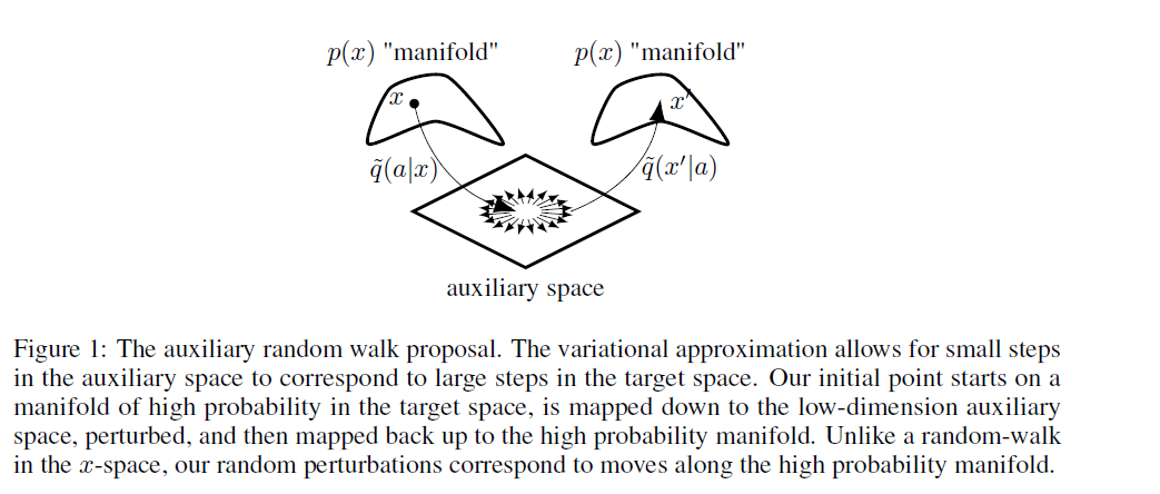
(2) Auxiliary Random Walk Proposal Distribution
Example 3) Auxiliary Random Walk Proposal Distribution
-
additional random perturbation in the auxiliary \(a\)-space
-
proposal : \(\tilde{q}\left(x^{\prime} \mid x\right)=\int q_{*}\left(x^{\prime} \mid a^{\prime}\right) \tilde{q}\left(a^{\prime} \mid a\right) p_{*}(a \mid x) d a d a^{\prime}\).
where \(\tilde{q}\left(a^{\prime} \mid a\right)=\mathcal{N}\left(a^{\prime} \mid a, \sigma_{a}^{2} I\right)\)
-
Summary
- 1) mapping from high-dim \(x\) to low-dim \(a\)
- 2) perform random walk in \(a\)-space
- 3) mapping back to high-dim space \(x\)
2-4. Choosing the Variational Family
Not finished yet! Have to decide the structure of variational distn, \(q(a, x)\) and \(p(a \mid x)\)
\(\rightarrow\) use DNN!
-
\(q(a) =\mathcal{N}(a \mid 0, I)\).
-
\(q_{\phi}(x \mid a) =\mathcal{N}\left(x \mid \mu_{\phi}(a), \Sigma_{\phi}(a)\right)\).
-
\(p_{\theta}(a \mid x) =\mathcal{N}\left(a \mid \mu_{\theta}(x), \Sigma_{\theta}(x)\right)\).
where \(q_{\phi}(x \mid a)\) and \(p_{\theta}(a \mid x)\) are diagonal Gaussian
Key to flexibility of the auxiliary variational method ?
\(\rightarrow\) while \(q(a,x)\) can be evaluated point-wise, the marginal \(q(x)\) is a much richer approximating distn
Algorithm Summary