(paper 7) Prototypical Contrastive Learning (PCL)

Prototypical Contrastive Learning of Unsupervised Representations

Contents

1. Abstract
2. Introduction
3. PCL (Prototypical Contrastive Learning)
   1. Preliminaries
   2. PCL as EM
   3. Concentration Estimation \(\phi\)

0. Abstract

Prototypical Contrastive Learning (PCL)

• bridge contrastive learning with clustering

• not only learns low-level features for the task of instance discrimination,

  but also encodes semantic structures discovered by clustering

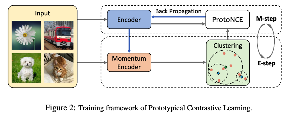
EM algorithm

[ E-step ] finding the distribution of prototypes via clustering

[ M-step ] optimizing the network via contrastive learning

ProtoNCE loss

• a generalized version of the InfoNCE loss for contrastive learning
• encourages representations to be closer to their assigned prototypes

1. Introduction

2. PCL (Prototypical Contrastive Learning)

(1) Preliminaries

Notation

• training set \(X=\left\{x_{1}, x_{2}, \ldots, x_{n}\right\}\) of \(n\) images
• embedding function \(f_{\theta}\)
  • map \(X\) to \(V=\left\{v_{1}, v_{2}, \ldots, v_{n}\right\}\) with \(v_{i}=f_{\theta}\left(x_{i}\right)\)

Instance-wise Contrastive Learning :

• optimize InfoNCE (ex)
• \(\mathcal{L}_{\text {InfoNCE }}=\sum_{i=1}^{n}-\log \frac{\exp \left(v_{i} \cdot v_{i}^{\prime} / \tau\right)}{\sum_{j=0}^{r} \exp \left(v_{i} \cdot v_{j}^{\prime} / \tau\right)}\).

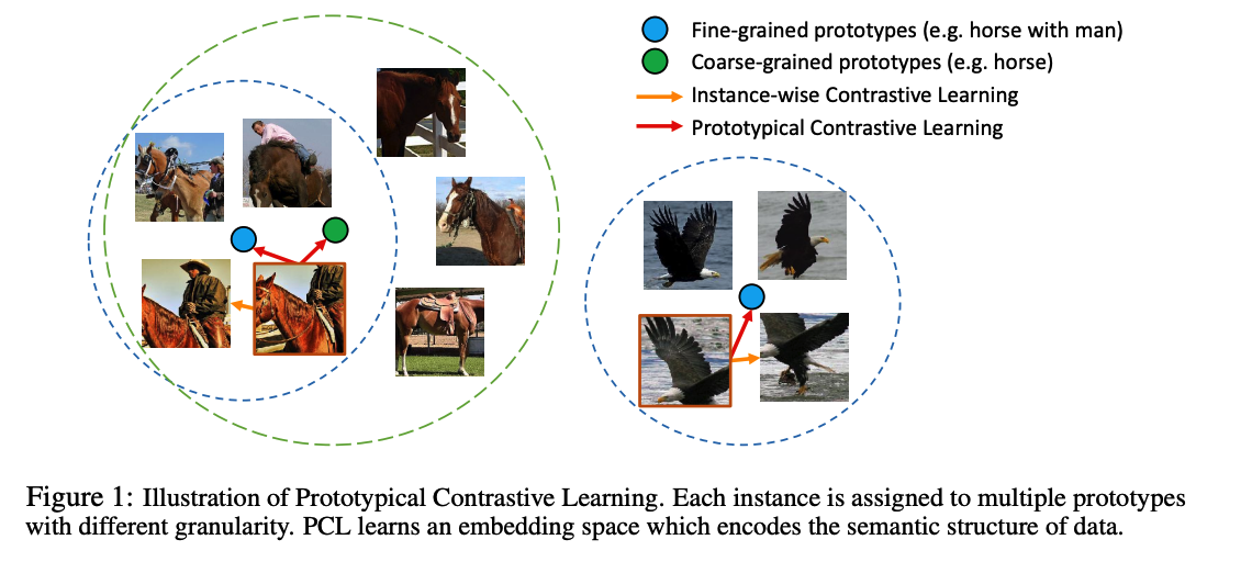
Prototypical Contrastive Learning

• use prototypes \(c\) instead of \(v^{\prime}\)

• replace the fixed temperature \(\tau\) with a per-prototype concentration estimation \(\phi\)

(2) PCL as EM

\(\theta^{*}=\underset{\theta}{\arg \max } \sum_{i=1}^{n} \log p\left(x_{i} ; \theta\right)=\underset{\theta}{\arg \max } \sum_{i=1}^{n} \log \sum_{c_{i} \in C} p\left(x_{i}, c_{i} ; \theta\right)\).

\(\rightarrow\) MLE : \(\theta^{*}=\underset{\theta}{\arg \min } \sum_{i=1}^{n}-\log \frac{\exp \left(v_{i} \cdot c_{s} / \phi_{s}\right)}{\sum_{j=1}^{k} \exp \left(v_{i} \cdot c_{j} / \phi_{j}\right)}\).

Loss Function

• take the same approach as NCE

  ( sample \(r\) negative prototypes to calculate the normalization term )

• also, cluster samples \(M\) times with different number of clusters \(K=\{k_m\}_{m=1}^M\)

• Add InfoNCE loss to retain the property of local smoothness

\(\mathcal{L}_{\text {ProtoNCE }}=\sum_{i=1}^{n}-\left(\log \frac{\exp \left(v_{i} \cdot v_{i}^{\prime} / \tau\right)}{\sum_{j=0}^{r} \exp \left(v_{i} \cdot v_{j}^{\prime} / \tau\right)}+\frac{1}{M} \sum_{m=1}^{M} \log \frac{\exp \left(v_{i} \cdot c_{s}^{m} / \phi_{s}^{m}\right)}{\sum_{j=0}^{r} \exp \left(v_{i} \cdot c_{j}^{m} / \phi_{j}^{m}\right)}\right)\).

(3) Concentration Estimation \(\phi\)

desired \(\phi\) : should be SMALL, if

• average distance between \(v_z^{'}\) and \(c\) is small

• cluster contains more feature points ( \(i.e. Z\) is large )

\(\phi=\frac{\sum_{z=1}^{Z} \mid \mid v_{z}^{\prime}-c \mid \mid _{2}}{Z \log (Z+\alpha)}\).