(paper 6) CSI

CSI: Novelty Detection via Contrastive Learning on Distributionally Shifted Instances

Contents

1. Abstract
2. Introduction
3. CSI : Contrasting Shifted Instances
   1. Contrastive Learning
   2. Contrastive Learning for Distribution-shifting transformations
   3. Score Functions for detecting OOD

0. Abstract

Novelty Detection

• check if data is from outside the training distn

This paper proposes a simple & effective method, called CSI ( Contrasting Shifted Instances )

( inspired by contrastive learning of visual representations)

• key : contrasts the sample with “distributionally-shifted augmentations” of itself

• propose a new detection score

1. Introduction

OOD detection = Novelty/Anomaly detection

\(\rightarrow\) is test data from training data distn ??

• (1) density based
• (2) reconstruction based
• (3) one-classifier
• (4) self-supervised

Majority of recent works :

• step 1) modeling the representation to better encode normality
• step 2) define a new detection score

Instance Discrimination

• special type of contrastive learning

OOD detection vs Standard Representation learning

• OOD ) discriminate in-distribution & OOD samples
• RL ) discriminate within in-distribution

Existing contrastive learning scheme is already reasonably effective for detecting OOD samples with a proper detection score

• ex) by using data augmentation

• (A) previous works

  • pull augmented samples

• (B) proposed

  • PUSH augmented samples!

  • found that contrasting shifted samples help OOD detection!

    able to both…

    • (1) discriminate between in & out distn
    • (2) (original task) discriminate within in-distn

Contributions of CSI

propose 2 novel additional components :

• (1) new training method, which contrasts distributionally-shifted augmentations!
  • augmented sample \(\neq\) same sample ( positive pair )
• (2) score function, which utilizes both
  • (a) contrastively learned representation
  • (b) new training method

2. CSI : Contrasting Shifted Instances

Notation

• dataset : \(\left\{x_{m}\right\}_{m=1}^{M}\) ~ \(p_{\text {data }}(x)\)
• data space : \(\mathcal{X}\)

Goal of OOD detection :

• whether \(x\) is from \(p_{\mathrm{data}}(x)\) or not
• modeling \(p_{\text {data }}(x)\) is prohibitive! \(\rightarrow\) define a score function \(s(x)\)
  • high score = from in-distribution

(1) Contrastive Learning

Goal :

• learn an encoder \(f_{\theta}\) to extract the necessary information to distinguish similar samples from the others!

Notation

• \(x\) : query
• \(\left\{x_{+}\right\}\) and \(\left\{x_{-}\right\}\) : set of positive and negative samples
• \(\operatorname{sim}\left(z, z^{\prime}\right):=z \cdot z^{\prime} / \mid \mid z \mid \mid \tilde{ \mid \mid } \mid \mid z^{\prime} \mid \mid\) : cosine similarity

Contrastive Loss :

• \(\mathcal{L}_{\text {con }}\left(x,\left\{x_{+}\right\},\left\{x_{-}\right\}\right):=-\frac{1}{ \mid \left\{x_{+}\right\} \mid } \log \frac{\sum_{x^{\prime} \in\left\{x_{+}\right\}} \exp \left(\operatorname{sim}\left(z(x), z\left(x^{\prime}\right)\right) / \tau\right)}{\sum_{x^{\prime} \in\left\{x_{+}\right\} \cup\left\{x_{-}\right\}} \exp \left(\operatorname{sim}\left(z(x), z\left(x^{\prime}\right)\right) / \tau\right)}\).
  • \(\left\{x_{+}\right\}, z(x)\) : the output feature of the contrastive layer

SimCLR

for Instance Discrimination

Notation :

• \(\tilde{x}_{i}^{(1)}\) & \(\tilde{x}_{i}^{(2)}\) : two augmented samples from \(x_i\)
  • \(\tilde{x}^{(1)}:=T_{1}\left(x_{i}\right)\).
  • \(\tilde{x}^{(2)}:=T_{2}\left(x_{i}\right)\).

SimCLR objective function :

• contrastive loss, where each \(\left(\tilde{x}_{i}^{(1)}, \tilde{x}_{i}^{(2)}\right)\) and \(\left(\tilde{x}_{i}^{(2)}, \tilde{x}_{i}^{(1)}\right)\) are considered as query-key pairs

  ( others = negatives )

• \(\mathcal{L}_{\text {SimCLR }}(\mathcal{B} ; \mathcal{T}):=\frac{1}{2 B} \sum_{i=1}^{B} \mathcal{L}_{\text {con }}\left(\tilde{x}_{i}^{(1)}, \tilde{x}_{i}^{(2)}, \tilde{\mathcal{B}}_{-i}\right)+\mathcal{L}_{\text {con }}\left(\tilde{x}_{i}^{(2)}, \tilde{x}_{i}^{(1)}, \tilde{\mathcal{B}}_{-i}\right)\).

  • where \(\tilde{\mathcal{B}}:=\left\{\tilde{x}_{i}^{(1)}\right\}_{i=1}^{B} \cup\left\{\tilde{x}_{i}^{(2)}\right\}_{i=1}^{B}\) and \(\tilde{\mathcal{B}}_{-i}:=\left\{\tilde{x}_{j}^{(1)}\right\}_{j \neq i} \cup\left\{\tilde{x}_{j}^{(2)}\right\}_{j \neq i}\).

(2) Contrastive Learning for Distribution-shifting transformations

Which transformation to use??

• Some augmentations (e.g., rotation) degrades the discriminative performance of SimCLR!

\(\rightarrow\) this paper, shows that some augmentations can be useful for OOD detection! ( by considering them as negatives )

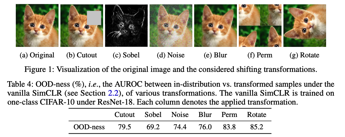
Family of augmentations \(S\)

• distribution-shifting transformations ( = shifting transformations )
• lead to better representation for OOD, when used as negatives

a) Contrasting Shifted Instances (CSI)

consider a set \(\mathcal{S}\) consisting of \(K\) different transformations

• \(\mathcal{S}:=\left\{S_{0}=I, S_{1}, \ldots, S_{K-1}\right\}\).

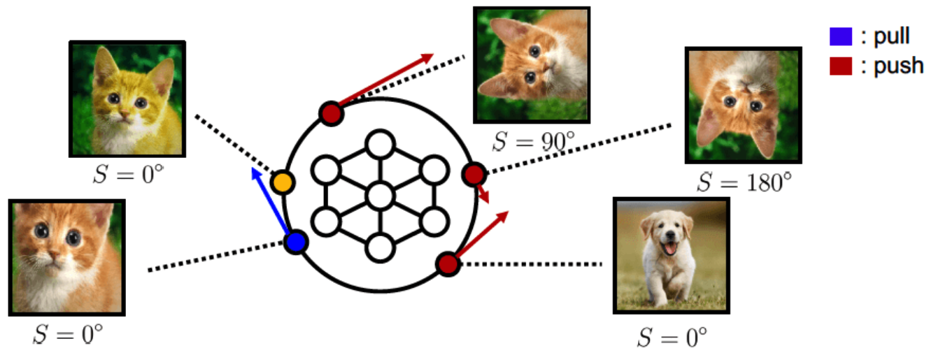
Vanilla SimCLR vs Proposed

• SimCLR : consider augmented as POSITIVE
• Proposed : consider augmented as NEGATIVE ( if it is from \(\mathcal{S}\) )

con-SI ( Contrasting Shifted Instances ) loss

• \(\mathcal{L}_{\text {con-SI }}:=\mathcal{L}_{\text {SimCLR }}\left(\bigcup_{S \in \mathcal{S}} \mathcal{B}_{S} ; \mathcal{T}\right), \quad \text { where } \mathcal{B}_{S}:=\left\{S\left(x_{i}\right)\right\}_{i=1}^{B} .\).

• intuition : regard each distributionally-shifted sample as OOD
• Discriminate (1) & (2)
  • (1) \(S=I\)
  • (2) \(S \in \{S_1, \cdots, S_{K-1}\}\).

\(\rightarrow\) improvement in OOD detection!

b) Classifying Shifted Instances

Auxiliary task

• auxiliary softmax classifier \(p_{\text {cls-SI }}\left(y^{\mathcal{S}} \mid x\right)\)

• predict which shifting transformation is applied ( \(y^{S} \in \mathcal{S}\) )

classifying shifted instances (cls-SI) loss

• \(\mathcal{L}_{\text {cls-SI }}:=\frac{1}{2 B} \frac{1}{K} \sum_{S \in \mathcal{S}} \sum_{\tilde{x}_{S} \in \tilde{\mathcal{B}}_{S}}-\log p_{\text {cls-SI }}\left(y^{\mathcal{S}}=S \mid \tilde{x}_{S}\right) .\).

a) + b) = Final Loss

combining the two objectives:

• \(\mathcal{L}_{\text {CSI }}=\mathcal{L}_{\text {con-SI }}+\lambda \cdot \mathcal{L}_{\text {cls-SI }}\).

( https://github.com/alinlab/CSI/blob/master/training/unsup/simclr_CSI.py )

images1 = torch.cat([P.shift_trans(images1, k) for k in range(P.K_shift)])
images2 = torch.cat([P.shift_trans(images2, k) for k in range(P.K_shift)])
shift_labels = torch.cat([torch.ones_like(labels) * k for k in
                          range(P.K_shift)], 0)  # B -> 4B
shift_labels = shift_labels.repeat(2)

images_pair = torch.cat([images1, images2], dim=0)  # 8B
images_pair = simclr_aug(images_pair)  # transform

_, outputs_aux = model(images_pair, simclr=True, penultimate=True, shift=True)

simclr = normalize(outputs_aux['simclr'])  # normalize
sim_matrix = get_similarity_matrix(simclr, multi_gpu=P.multi_gpu)
loss_sim = NT_xent(sim_matrix, temperature=0.5) * P.sim_lambda

loss_shift = criterion(outputs_aux['shift'], shift_labels)

### total loss ###
loss = loss_sim + loss_shift

(3) Score Functions for detecting OOD

1) propose a detection score

2) introduce how to incorporate additional info learned by CSI

1) Detection Score

• 2 features from SimCLR : effective for detecting OOD samples
  • feature # 1) \(\max _{m} \operatorname{sim}\left(z\left(x_{m}\right), z(x)\right)\)
  • feature # 2) \(\mid \mid z(x) \mid \mid\)

\(\rightarrow\) contrastive loss increases \(\mid \mid z(x) \mid \mid\) of in-distn

( \(\because\) easy way to minimize cosine similarity of identical samples )

Thus, propose a simple detection score

• \(s_{\text {con }}\left(x ;\left\{x_{m}\right\}\right):=\max _{m} \operatorname{sim}\left(z\left(x_{m}\right), z(x)\right) \cdot \mid \mid z(x) \mid \mid\).

2) using CSI info in score

improve the \(s_{\text {con }}\) significantly by incorporating shifting transformations \(\mathcal{S}\).

proposes 2 additional scores

• (1) \(s_{\text {con-SI }}\)
• (2) \(s_{\text {cls-SI }}\)

\(s_{\text {con-SI }}\left(x ;\left\{x_{m}\right\}\right):=\sum_{S \in \mathcal{S}} \lambda_{S}^{\text {con }} s_{\text {con }}\left(S(x) ;\left\{S\left(x_{m}\right)\right\}\right)\).

• \[\lambda_{S}^{\text {con }}:=M / \sum_{m} s_{\text {con }}\left(S\left(x_{m}\right) ;\left\{S\left(x_{m}\right)\right\}\right)=M / \sum_{m} \mid \mid z\left(S\left(x_{m}\right)\right) \mid \mid\]
• expectation over \(\mathcal{S}\)

\(s_{\text {cls-SI }}(x):=\sum_{S \in \mathcal{S}} \lambda_{S}^{c 1 \mathrm{~s}} W_{S} f_{\theta}(S(x))\).

• where \(\lambda_{S}^{\text {c1s }}:=M / \sum_{m}\left[W_{S} f_{\theta}\left(S\left(x_{m}\right)\right)\right]\)
  • \(W_{S}\) : weight vector in the linear layer of \(p\left(y^{\mathcal{S}} \mid x\right)\) per \(S \in \mathcal{S}\).
• expectation over \(\mathcal{S}\)

Combined score for CSI representation :

• \(s_{\mathrm{CSI}}\left(x ;\left\{x_{m}\right\}\right):=s_{\text {con-SI }}\left(x ;\left\{x_{m}\right\}\right)+s_{\text {cls-SI }}(x)\).