DeepDPM : Deep Clustering With an Unknown Number of Clusters
Contents
- Abstract
- Introduction
- DPGMM-based Clustering
- Notation
- classical GMM
- split/merge fraemwork
- DeepDPM
- DeepDPM under fixed \(K\)
- Changing \(K\) via Splits and Merges
- Amortized EM Inference
- Weak Prior
- Feature Extraction
- Results
0. Abstract
Comparison
-
Classical Clustering : benefits from NON-parametric approach
-
DL Clustering : require a pre-defined number of clusters ( = \(K\) )
-
When \(K\) is unknown…. model selection?
\(\rightarrow\) computationally expensive
-
Propose DeepDPM
-
introduce an effective deep-clustering method, that does not require knowing value \(K\)
- (1) SPLIT/MERGE framework
- dynamic architecture, that adapts to the changing \(K\)
- (2) novel loss
1. Introduction
DL Clustering
- cluster large & high-dim datasets better & more efficiently
Classical Clustering :
- non-parametric methods have advantages!
DPM (Dirichlet Process Mxiture)
- [PROS] offer an elegant, data-adaptive, and mathematically-principled solution for clustering when \(K\) is unknown
- [CONS] high computational cost when inference
DeepDPM
effective deep non-parametric method
Practical Benefits of ability to infer the latent \(K\) :
- (1) without good estimate of \(K\), parametric methods suffer in performance!
- (2) changing \(K\) during training has positive optimization-related implications :
- by splitting one cluster into two, multiple data labels are changed simultaneously
- (3) finding \(K\) with model selection \(\rightarrow\) computationally expensive
- (4) \(K\) itself may be sought-after quantity of importance
Details of DPM
-
combine DL + DPM
-
use split & merge to change \(k\)
- use novel amortized inference for EM algorithms in mixture models
- differentiable during most of training ( except split & merge )
2. DPGMM-based Clustering
(1) Notation
- \(\mathcal{X}=\left(\boldsymbol{x}_{i}\right)_{i=1}^{N}\) : \(N\) data points of \(d\) dimension
- clustering task : partition \(\mathcal{X}\) into \(K\) disjoint groups
- \(z_{i}\) : cluster label of \(\boldsymbol{x}_{i}\)
- data of certain cluster : \(\left(\boldsymbol{x}_{i}\right)_{i: z_{i}=k}\)
(2) classical GMM
DPGMM (a specific case of the DPM) :
- mixture with infinitely-many Gaussians
- often used, when \(K\) is unknown
- \(p\left(\boldsymbol{x} \mid\left(\boldsymbol{\mu}_{k}, \boldsymbol{\Sigma}_{k}, \pi_{k}\right)_{k=1}^{\infty}\right)=\sum_{k=1}^{\infty} \pi_{k} \mathcal{N}\left(\boldsymbol{x} ; \boldsymbol{\mu}_{k}, \boldsymbol{\Sigma}_{k}\right)\).
Component : \(\boldsymbol{\theta}_{k}=\left(\boldsymbol{\mu}_{k}, \boldsymbol{\Sigma}_{k}\right)\)
- \(\boldsymbol{\theta}=\left(\boldsymbol{\theta}_{k}\right)_{k=1}^{\infty}\).
- \(\boldsymbol{\pi}=\left(\pi_{k}\right)_{k=1}^{\infty}\).
- assumed to be drawn from their own prior
(3) split/merge fraemwork
augments latent variables with auxilairy variables
-
latent variables : \(\left(\boldsymbol{\theta}_{k}\right)_{k=1}^{\infty}, \boldsymbol{\pi}\) , \(\left(z_{i}\right)_{i=1}^{N}\)
-
auxiliary variables :
-
to each \(z_{i}\), an additional subcluster label, \(\widetilde{z}_{i} \in\{1,2\}\), is added.
-
to each \(\boldsymbol{\theta}_{k}\), two subcomponents are added, \(\widetilde{\boldsymbol{\theta}}_{k, 1}, \widetilde{\boldsymbol{\theta}}_{k, 2}\), with nonnegative weights \(\widetilde{\pi}_{k}=\left(\widetilde{\pi}_{k, j}\right)_{j \in\{1,2\}}\)
- where \(\widetilde{\pi}_{k, 1}+\widetilde{\pi}_{k, 2}=1\)
\(\rightarrow\) 2-component GMM
-
MH-framework
-
allow changing \(K\) during training
-
split of cluster \(k\) into its subclusters is proposed
-
split acceptance ratio :
- \(H_{\mathrm{s}}=\frac{\alpha \Gamma\left(N_{k, 1}\right) f_{\boldsymbol{x}}\left(\mathcal{X}_{k, 1} ; \lambda\right) \Gamma\left(N_{k, 2}\right) f_{\boldsymbol{x}}\left(\mathcal{X}_{k, 2} ; \lambda\right)}{\Gamma\left(N_{k}\right) f_{\boldsymbol{x}}\left(\mathcal{X}_{k} ; \lambda\right)}\).
- \(\mathcal{X}_{k}=\left(\boldsymbol{x}_{i}\right)_{i: z_{i}=k}\) : points in cluster \(k\)
- \(N_{k}= \mid \mathcal{X}_{k} \mid\) : number of points in cluster \(k\)
- \(f_{\boldsymbol{x}}(\cdot ; \lambda)\) : marginal likelihood
- interpretation : comparing the marginal likelihood of the data, under 2 subclusters with its marginal likelihood under the cluster
- \(H_{\mathrm{s}}=\frac{\alpha \Gamma\left(N_{k, 1}\right) f_{\boldsymbol{x}}\left(\mathcal{X}_{k, 1} ; \lambda\right) \Gamma\left(N_{k, 2}\right) f_{\boldsymbol{x}}\left(\mathcal{X}_{k, 2} ; \lambda\right)}{\Gamma\left(N_{k}\right) f_{\boldsymbol{x}}\left(\mathcal{X}_{k} ; \lambda\right)}\).
3. DeepDPM
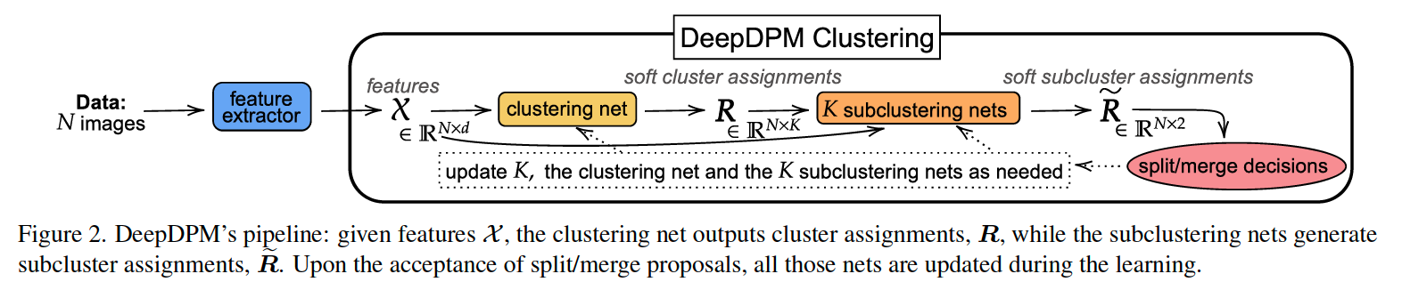
2 main parts :
- (1) clustering net
- (2) \(K\) subclustering nets ( one for each cluster )
(1) DeepDPM under fixed \(K\)
a) Clustering Net ( \(f_{\mathrm{cl}}\) )
\(f_{\mathrm{cl}}(\mathcal{X})=\boldsymbol{R}=\left(\boldsymbol{r}_{i}\right)_{i=1}^{N} \quad \boldsymbol{r}_{i}=\left(r_{i, k}\right)_{k=1}^{K}\).
- for each data point \(\boldsymbol{x}_{i}\), generate \(K\) soft cluster assignments
- where \(r_{i, k} \in[0,1]\) is the soft assignment ( \(\sum_{k=1}^{K} r_{i, k}=1\) )
Hard assignment
-
from (soft) \(\left(\boldsymbol{r}_{i}\right)_{i=1}^{N}\), compute (hard) \(\boldsymbol{z}=\left(z_{i}\right)_{i=1}^{N}\)
( \(z_{i}=\arg \max _{k} r_{i, k}\) )
b) Subclustering Net ( \(f_{\text {sub }}^{k}\) )
\(f_{\text {sub }}^{k}\left(\mathcal{X}_{k}\right)=\widetilde{\boldsymbol{R}}_{k}=\left(\widetilde{\boldsymbol{r}}_{i}\right)_{i: z_{i}=k} \quad \widetilde{\boldsymbol{r}}_{i}=\left(\widetilde{r}_{i, j}\right)_{j=1}^{2}\).
-
\(\boldsymbol{z}=\left(z_{i}\right)_{i=1}^{N}\) is fed into \(f_{\text {sub }}^{k}\) ( to its respective cluster )
\(\rightarrow\) generates soft subcluster assignments
-
where \(\widetilde{r}_{i, j} \in[0,1]\) is the soft assignment of \(\boldsymbol{x}_{i}\) to subcluster \(j(j \in\{1,2\})\)
- \(\widetilde{r}_{i, 1}+\widetilde{r}_{i, 2}=1\).
Subclusters learned by \(\left(f_{\text {sub }}^{k}\right)_{k=1}^{K}\) are used in split proposals.
c) MLP
Each of the \(K+1\) nets \(\left(f_{\text {cl }}\right.\) and \(\left(f_{\text {sub }}^{k}\right)_{k=1}^{K}\) ) :
-
MLP with single hidden layer
-
Neurons of last layer :
- \(f_{\mathrm{cl}}\) : \(K\) neurons
- each \(f_{\text {sub }}^{k}\) : \(2\) neurons
d) New Loss
motivated by EM in Bayesian GMM
[ E-step ]
- For each \(\boldsymbol{x}_{i}\) and each \(k \in\{1, \ldots, K\}\) , compute E-step probabilities \(\boldsymbol{r}_{i}^{\mathrm{E}}=\left(r_{i, k}^{\mathrm{E}}\right)_{k=1}^{K}\)
- \(r_{i, k}^{\mathrm{E}}=\frac{\pi_{k} \mathcal{N}\left(\boldsymbol{x}_{i} ; \boldsymbol{\mu}_{k}, \boldsymbol{\Sigma}_{k}\right)}{\sum_{k^{\prime}=1}^{K} \pi_{k^{\prime}} \mathcal{N}\left(\boldsymbol{x}_{i} ; \boldsymbol{\mu}_{k^{\prime}}, \boldsymbol{\Sigma}_{k^{\prime}}\right)} \quad k \in\{1, \ldots, K\}\).
- computed using \(\left(\pi_{k}, \boldsymbol{\mu}_{k}, \boldsymbol{\Sigma}_{k}\right)_{k=1}^{K}\) from previous epochs
encourage \(f_{\text {cl }}\) to generate similar soft assignments using the following new loss:
- \(\mathcal{L}_{\mathrm{cl}}=\sum_{i=1}^{N} \mathrm{KL}\left(\boldsymbol{r}_{i} \mid \mid \boldsymbol{r}_{i}^{\mathrm{E}}\right)\).
[ M-step ]
-
uses the weighted versions of the MAP estimates of \(\left(\pi_{k}, \boldsymbol{\mu}_{k}, \boldsymbol{\Sigma}_{k}\right)_{k=1}^{K}\) ,
where the weights are…
- \(r_{i, k}^{\mathrm{E}}\) (X)
- \(r_{i, k}\) (O) \(\rightarrow\) output of \(f_{cl}\)
for \(\left(f_{\text {sub }}^{k}\right)_{k=1}^{K}\) … calculate Isotropic Loss :
- \(\mathcal{L}_{\text {sub }}=\sum_{k=1}^{K} \sum_{i=1}^{N_{k}} \sum_{j=1}^{2} \widetilde{r}_{i, j} \mid \mid \boldsymbol{x}_{i}-\widetilde{\boldsymbol{\mu}}_{k, j} \mid \mid _{\ell_{2}}^{2}\).
- where \(N_{k}= \mid \mathcal{X}_{k} \mid\)
- \(\tilde{\boldsymbol{\mu}}_{k, j}\) : mean of subcluster \(j\) of cluster \(k\)
(2) Changing \(K\) via Splits and Merges
Every few epochs, propose either SPLITS or MERGES
= K changes !
= last layer of \(K+1\) nets changes !
a) Splits
propose to split each of the clusters into 2 subclusters
- split probability = \(\min (1, H_{\mathrm{s}} )\)
IF ACCEPTED ( = SPLIT ) for cluster \(k\)…
-
(Clustering Net) \(k\)-th unit of last layer is duplicated
- initialize the parameters of 2 new clusters, with parametes of SUBcluster nets
- \(\begin{array}{lll} \boldsymbol{\mu}_{k_{1}} \leftarrow \widetilde{\boldsymbol{\mu}}_{k, 1}, & \boldsymbol{\Sigma}_{k_{1}} \leftarrow \widetilde{\boldsymbol{\Sigma}}_{k, 1}, & \pi_{k_{1}} \leftarrow \pi_{k} \times \widetilde{\boldsymbol{\pi}}_{k, 1} \\ \boldsymbol{\mu}_{k_{2}} \leftarrow \widetilde{\boldsymbol{\mu}}_{k, 2}, & \boldsymbol{\Sigma}_{k_{2}} \leftarrow \widetilde{\boldsymbol{\Sigma}}_{k, 2}, & \pi_{k_{2}} \leftarrow \pi_{k} \times \widetilde{\boldsymbol{\pi}}_{k, 2} \end{array}\).
- \(k_{1}\) and \(k_{2}\) : indices of the new clusters
- initialize the parameters of 2 new clusters, with parametes of SUBcluster nets
b) Merges
Splits vs Merge
- Splits : can be done in parallel
- Merge : cannot ~
To avoid sequentially considering all possible merges…
\(\rightarrow\) merges of each cluster with only its 3 nearest neighbors
Merge probability : \(H_{\mathrm{m}}=1 / H_{\mathrm{s}}\)
IF ACCEPTED ( = MERGE ) …
- 2 clusters are merged
- new subcluster network of the merged clusters is made
- one of the 2 clusters’ weight (connected to the last layer) is removed from \(f_{cl}\)
(3) Amortized EM Inference
learned from data!
better than ground-truth \(K\)
(4) Weak Prior
intentially choose the prior to be very weak!
(5) Feature Extraction
to show the effectiveness… use 2 types of FE paradigms
- (1) end-to-end
- features & clustering are jointly learned
- (2) 2-step appraoch
- features are learned once & held fixed
- 2 step :
- MoCo ( for feature extraction )
- SCAN ( for clustering )
4. Results
3 common metrics ( higher = better )
- clustering accuracy (ACC)
- Normalized Mutual Information(NMI)
- Adjusted Rand Index (ARI).
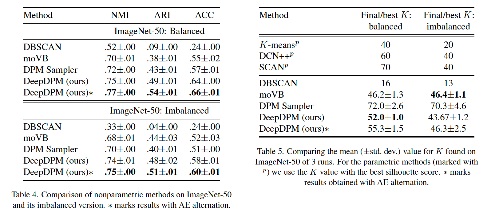
(1) Comparison with classical methods
parametric : K-means, GMM
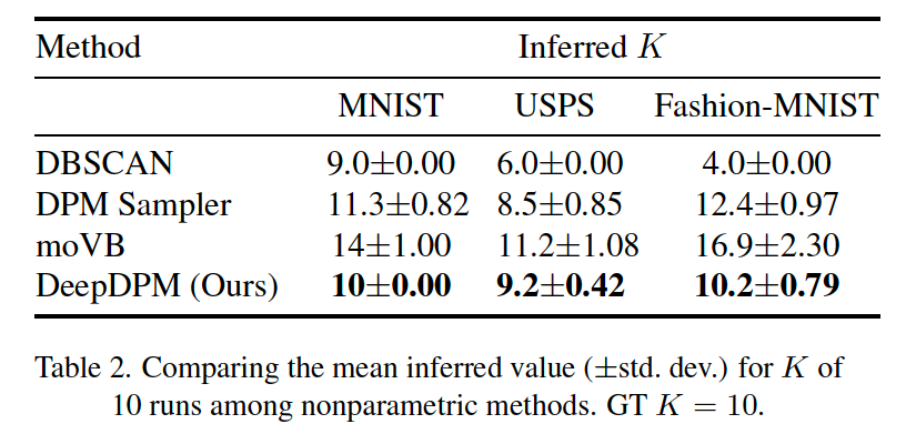
nonparametric : DBSCAN, moVB, DPM sampler
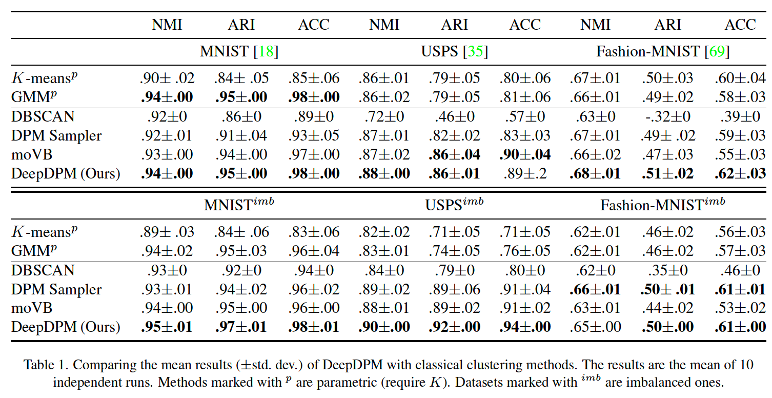
among the nonparametric methods, DeepDPM’s inferred \(K\) is the closest to the GT \(K\)
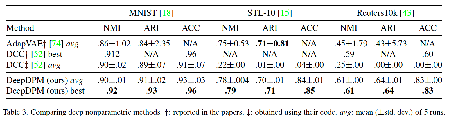
(2) Comparison with Deep Nonparametric methods
there exist very few deep nonparametric methods
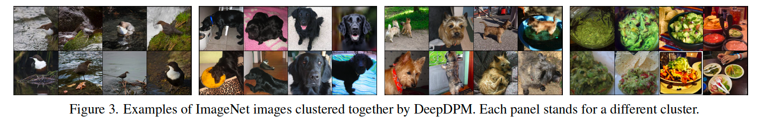
(3) Clustering the Entire ImageNet Dataset
initialized with \(K = 200\), and converged into \(707\) clusters ( GT = \(1000\) ).
(4) Class-imbalance
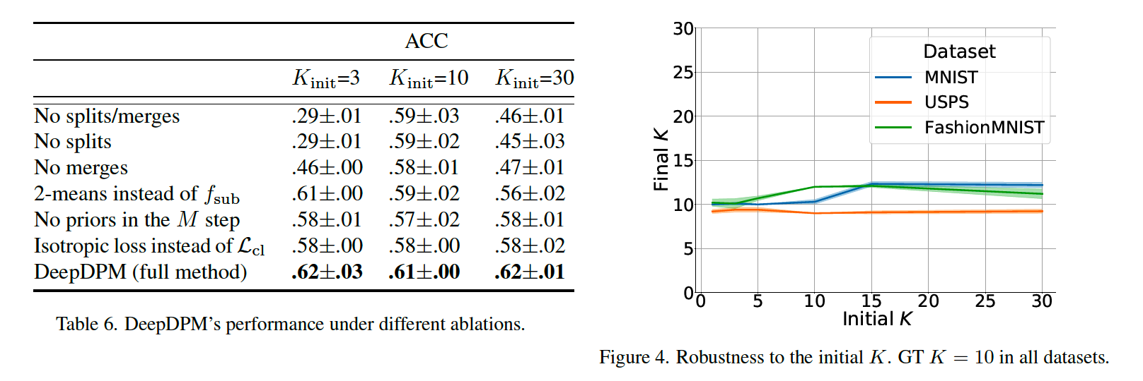
(5) Ablation Study