mixup: Beyound Empirical Risk MinimizationPermalink

( https://arxiv.org/pdf/1710.09412.pdf )

ContentsPermalink

1. Abstract
2. Introduction
   1. Properties of ERM
   2. VRM / DA
   3. Mixup
3. from ERM to Mixup
   1. VRM
   2. Contribution

0. AbstractPermalink

problem of DL

• memorization
• sensitivity to adversarial examples

$\rightarrow$ propose mixup

Mixup

• trains NN on convex combinations of (x,y) pairs
• regularizes NN to favor simple linear behavior in-between training examples

1. IntroductionPermalink

NN share two commonalities.

1. trained to minimize their average error over the training data

   ( = Empirical Risk Minimization (ERM) principle )

2. size of SOTA NN scales linearly with the number of training examples ( = N )

( classical result in learning theory ) convergence of ERM is guaranteed as long as the size of the learning machine does not increase with N

• size of a learning machine : measured in terms of its number of parameters ( or VC-complexity )

Properties of ERMPermalink

(1) ERM allows large NN to memorize the training data

• even in the presence of strong regularization
• even in classification problems where the labels are assigned at random

(2) NN trained with ERM change their predictions drastically when evaluated on OOD ( = adversarial examples )

$\rightarrow$ ERM is unable to explain or provide generalization on testing distributions that differ only slightly from the training data

Then… alternative of ERM??

VRM / DAPermalink

• Data Augmentation (DA) : formalized by the Vicinal Risk Minimization (VRM) principle

• in VRM, human knowledge is required to describe a vicinity or neighborhood around each example in the training data

  $\rightarrow$ draw additional virtual examples from the vicinity distribution of the training examples

  $\rightarrow$ enlarge the support of the training distribution.

• example ) CV

  • common to define the vicinity of one image as the set of its horizontal reflections, slight rotations, and mild scalings

• while DA leads to improved generalization …..

  • dataset-dependent & requires expert knowledge.

  • assumes that examples in the vicinity share the same class,

    & does not model the vicinity relation across examples of different classes

MixupPermalink

introduce a simple and data-agnostic DA

constructs virtual training examples as …

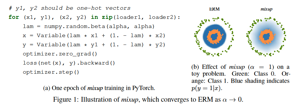
$\begin{array}{ll} \tilde{x}=\lambda x_i+(1-\lambda) x_j, & \text { where } x_i, x_j \text { are raw input vectors } \\ \tilde{y}=\lambda y_i+(1-\lambda) y_j, & \text { where } y_i, y_j \text { are one-hot label encodings } \end{array}$.

Summary

• extends the training distribution by incorporating the prior knowledge that…

  linear interpolations of feature vectors should lead to linear interpolations of the associated targets

2. from ERM to MixupPermalink

Supervised learning :

• find a function $f \in \mathcal{F}$
  • that describes the relationship between a $X$ and $Y$, which follow the joint distribution $P(X, Y)$.

• define a loss function $\ell$

  • that penalizes the differences between $f(x)$ and $y$, for $(x, y) \sim P$.

• minimize the average of the loss function $\ell$ over the data distribution $P$,

  ( = Expected Risk , $R(f)=\int \ell(f(x), y) \mathrm{d} P(x, y)$ )

Distribution $P$ is unknown!

• instead, have access to a set of training data $\mathcal{D}=\left\{\left(x_i, y_i\right)\right\}_{i=1}^n$, where $\left(x_i, y_i\right) \sim P$
• approximate $P$ by the empirical distribution
  • $P_\delta(x, y)=\frac{1}{n} \sum_{i=1}^n \delta\left(x=x_i, y=y_i\right)$.
    • where $\delta\left(x=x_i, y=y_i\right)$ is a Dirac mass centered at $\left(x_i, y_i\right)$.
  • using the $P_\delta$, approximate the expected risk by the empirical risk
    • $R_\delta(f)=\int \ell(f(x), y) \mathrm{d} P_\delta(x, y)=\frac{1}{n} \sum_{i=1}^n \ell\left(f\left(x_i\right), y_i\right)$.

$\rightarrow$ Empirical Risk Minimization (ERM) principle

Pros & Cons

• [pros] efficient to compute

• [cons] monitors the behaviour of $f$ only at a finite set of $n$ examples

  $\rightarrow$ trivial way : memorize the training data ( = overfitting )

Naïve estimate $P_\delta$ is one out of many possible choices to approximate the true distribution P.

• ex) Vicinal Risk Minimization (VRM)

VRMPermalink

• distn $P$ is approximated by $P_\nu(\tilde{x}, \tilde{y})=\frac{1}{n} \sum_{i=1}^n \nu\left(\tilde{x}, \tilde{y} \mid x_i, y_i\right)$.
• $\nu$ : a vicinity distribution
  • measures the probability of finding the virtual feature-target pair $(\tilde{x}, \tilde{y})$ in the vicinity of the training feature-target pair $\left(x_i, y_i\right)$.
• ex 1) Gaussian vicinities
  • $\nu\left(\tilde{x}, \tilde{y} \mid x_i, y_i\right)=\mathcal{N}\left(\tilde{x}-x_i, \sigma^2\right) \delta\left(\tilde{y}=y_i\right)$,
  • which is equivalent to augmenting the training data with additive Gaussian noise.

To learn using VRM …

• (1) sample the vicinal distribution to construct a dataset $\mathcal{D}_\nu:=\left\{\left(\tilde{x}_i, \tilde{y}_i\right)\right\}_{i=1}^m$,
• (2) minimize the empirical vicinal risk: $R_\nu(f)=\frac{1}{m} \sum_{i=1}^m \ell\left(f\left(\tilde{x}_i\right), \tilde{y}_i\right)$.

Contribution of this paperPermalink

propose a generic vicinal distribution

$\mu\left(\tilde{x}, \tilde{y} \mid x_i, y_i\right)=\frac{1}{n} \sum_j^n \underset{\lambda}{\mathbb{E}}\left[\delta\left(\tilde{x}=\lambda \cdot x_i+(1-\lambda) \cdot x_j, \tilde{y}=\lambda \cdot y_i+(1-\lambda) \cdot y_j\right)\right]$.

• where $\lambda \sim \operatorname{Beta}(\alpha, \alpha)$, for $\alpha \in(0, \infty)$.

  • $\alpha$ controls the strength of interpolation between feature-target pairs

    ( recovers the ERM principle as $\alpha \rightarrow 0$ )

• $\tilde{x}=\lambda x_i+(1-\lambda) x_j$.

• $\tilde{y}=\lambda y_i+(1-\lambda) y_j$.

recovering the ERM principle as $\alpha \rightarrow 0$.