(paper) SimMTM; A Simple Pre-Training Framework for Masked Time-Series Modeling

SimMTM: A Simple Pre-Training Framework for Masked Time-Series Modeling

( https://arxiv.org/abs/2302.00861.pdf )

Contents

1. Abstract
2. Introduction

0. Abstract

Mainstream paradigm : masked modeling

However, semantic information of TS is mainly contained in temporal variations … random masking : ruin vital temporal variations

\(\rightarrow\) present SimMTM

SimMTM

Simple pre-training framework for Masked Time-series Modeling

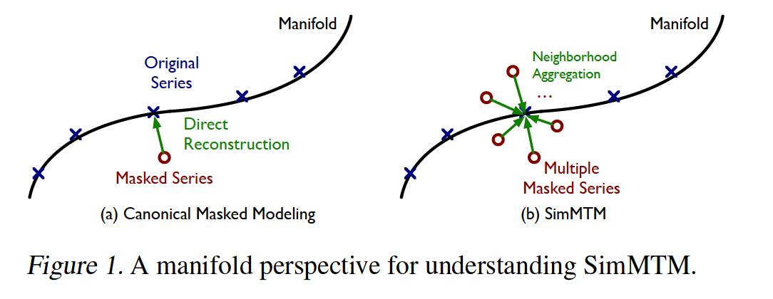
• relate masked modeling to manifold learning,

• proposes to recover masked time points
  • by the weighted aggregation of multiple neighbors outside the manifold
• learns to uncover the local structure of the manifold

Experiments

• (1) forecasting
• (2) classification

1. Introduction

Extends pre-training methods to TS

\(\rightarrow\) masked time-series modeling (MTM).

NLP & CV

• whose patches or words contain abundant even redundant semantic information

TS

• valuable semantic information of TS is mainly contained in the temporal variations
• ex) trend, periodicity and peak valley

\(\therefore\) Directly masking a portion of time points

\(\rightarrow\) ruin the temporal variations of the original TS

SimMTM

• randomly masked TS = “Neighbors” of original TS
• Reconstruction = project masked TS to original TS

But, direct reconstrution : fail due to random masking…

\(\rightarrow\) propose an idea as reconstructing the original TS from its MULTIPLE neighbors

Temporal variations of the original TS have been partially dropped in each randomly masked series

\(\rightarrow\) MULTIPLE randomly masked series will complement each other!

Process will also pre-train the model to uncover the local structure of the TS manifold implicitly

\(\rightarrow\) benefit masked modeling & representation learning

Details

• presents a neighborhood aggregation design for reconstruction
• aggregate the point-wise representations of TS
  • based on the similarities learned in the series-wise representation space.
• Losses
  • reconstruction loss
  • constraint loss
    • to guide the series-wise representation learning based on the neighborhood assumption of the TS manifold

Experiments

• achieves SOTA, when fine-tuning the pre-trained model into downstream tasks

• covers both …

  • ( low-level ) Forecasting

  • ( high-level ) Classification

2. Related Works

(1) SSL Pre-training : Contrastive Learning in TS

many designs of POS & NEG

TimCLR (Yang et al., 2022)

• adopts the DTW to generate phase-shift and amplitude change augmentations

TS2Vec (Yue et al., 2022)

• splits multiple time series into several patches
• defines the contrastive loss in both …
  • instance-wise
  • patch-wise

TS-TCC (Eldele et al., 2021)

• presents a new temporal contrastive learning task
  • make the augmentations predict each other’s future

TF-C (Zhang et al., 2022)

• proposes a novel time-frequency consistency architecture and
• optimizes time-based & frequency-based representations of the same example to be close to each other

Mixing-up (Wickstrøm et al., 2022)

• new samples are generated by mixing 2 data samples

• optimized to predict the mixing weights.

Summary

• CL mainly focuses on the high-level information (Xie et al., 2022a)
• series-wise / patch-wise representations inherently mismatch the lowlevel tasks ( ex) TS forecasting )

Thus, focus on the masked modeling paradigm

(2) SSL Pre-training : Masked Modeling in TS

Idea : optimizes the model by learning to reconstruct the masked content from unmasked part

TST (Zerveas et al., 2021)

• directly adopts the canonical masked modeling paradigm

  ( predict the removed time points based on the remaining time points )

PatchTST (Nie et al., 2022)

• learns to predict the masked subseries-level patches to capture the local semantic information
• reduce memory usage

[ Problem ]

directly masking time series

= ruin the essential temporal variations,

= makes the reconstruction too difficult to guide the representation learning

SimMTM

• direct reconstruction in previous works (X)
• reconstructing the original time series from multiple randomly masked series

(3) Understanding Masked Modeling

Masked modeling has been explored in stacked denoising autoencoders (Vincent et al., 2010)

Concepts

• Masking = adding noise to the original data
• Masked modeling = project the masked data from the neighborhood back to the original manifold ( = denoising )

Inspired by the manifold perspective…

• go beyond the classical denoising process
• project the masked data back to the manifold by aggregating multiple masked TS within the neighborhood.

3. SimMTM

proposes to reconstruct the original TS from multiple masked TS

step 1) learns similarities among multiple TS in the “series-wise” representation space

step 2) aggregates the point-wise representations of these TS

• based on the pre-learned “series-wise similarities”

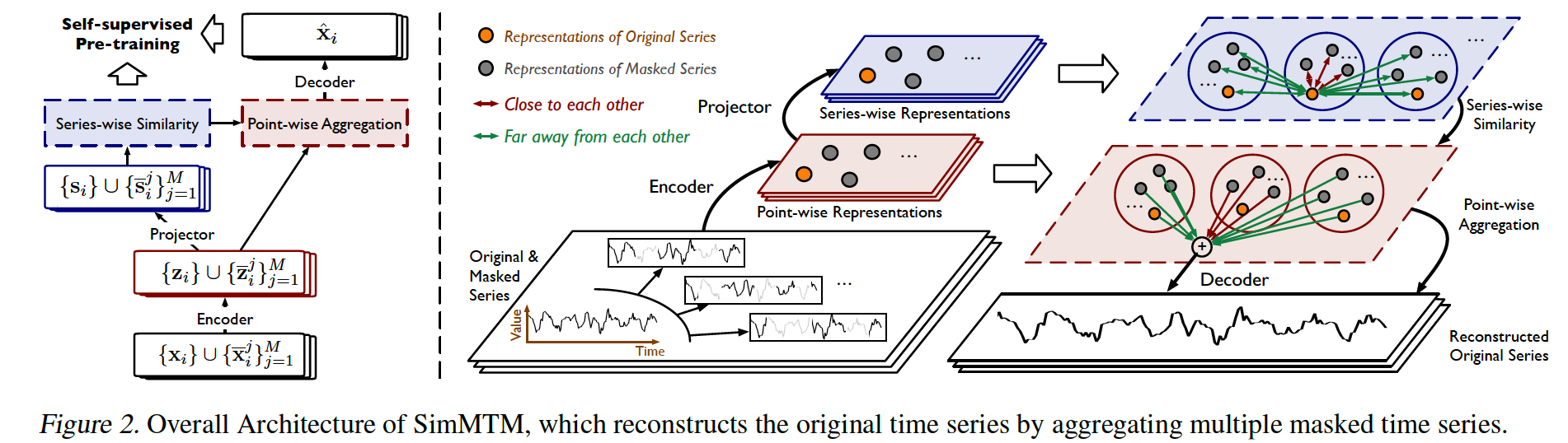
(1) Overall Architecture

involves the following 4modules:

• masking
• representation learning

• series-wise similarity learning

• point-wise reconstruction.

a) Masking

Input : \(\left\{\mathrm{x}_i\right\}_{i=1}^N\)

• mini-batch of \(N\) time series
• \(\mathbf{x}_i \in \mathbb{R}^{L \times C}\) : \(L\) time points and \(C\) observed variates

Output : \(\left\{\overline{\mathbf{x}}_i^j\right\}_{j=1}^M=\operatorname{Mask}_r\left(\mathbf{x}_i\right)\)

• set of masked series for each sample \(\mathbf{x}_i\)
  • by randomly masking a portion of time points
• \(r \in[0,1]\) : the masked portion
• \(M\) : hyperparameter for the number of masked TS
• \(\overline{\mathbf{x}}_i^j \in \mathbb{R}^{L \times C}\) : the \(j\)-th masked TS of \(\mathbf{x}_i\)

Batch of augmented TS

\(\mathcal{X}=\bigcup_{i=1}^N\left(\left\{\mathbf{x}_i\right\} \cup\left\{\overline{\mathbf{x}}_i^j\right\}_{j=1}^M\right)\).

• \((N \times(M+1))\) input series

b) Representation learning.

via encoder and projector layer, obtain …

• point-wise representations \(\mathcal{Z}\)

• series-wise representations \(\mathcal{S}\)

\(\begin{aligned} \mathcal{Z} & =\bigcup_{i=1}^N\left(\left\{\mathbf{z}_i\right\} \cup\left\{\overline{\mathbf{z}}_i^j\right\}_{j=1}^M\right)=\operatorname{Enocder}(\mathcal{X}) \\ \mathcal{S} & =\bigcup_{i=1}^N\left(\left\{\mathbf{s}_i\right\} \cup\left\{\overline{\mathbf{s}}_i^j\right\}_{j=1}^M\right)=\text { Projector }(\mathcal{Z}), \end{aligned}\).

• \(\mathbf{z}_i, \overline{\mathbf{z}}_i^j \in \mathbb{R}^{L \times d_{\text {model }}}\).
• \(\mathbf{s}_i, \overline{\mathbf{s}}_i^j \in \mathbb{R}^{1 \times d_{\text {model }}}\).

Architecturre

• (1) Encoder : encoder part of Transformer
  • will be transferred to downstream tasks during the fine-tuning process.
• (2) Projector : simple MLP layer along the temporal dimension
  • obtain series-wise representations

c) Series-wise similarity learning.

Directly averaging multiple masked TS

\(\rightarrow\) oversmoothing problem (Vincent et al., 2010)

Solution : \(\mathbf{R}=\operatorname{Sim}(\mathcal{S})\)

• \(\mathbf{R} \in \mathbb{R}^{(N \times(M+1)) \times(N \times(M+1))}\).
  • matrix of pairwise similarities for \((N \times(M+1))\) input samples
• utilize the similarities among series-wise representations \(\mathcal{S}\) for weighted aggregation
  • measured by the cosine distance ( \(\mathbf{R}_{\mathbf{u}, \mathbf{v}}=\frac{\mathbf{u v}^{\top}}{ \mid \mathbf{u} \mid \mid \mathbf{v} \mid }\) )
  • exploiting the local structure of the TS manifold.

d) Point-wise aggregation.

based on the learned series-wise similarities

Aggregation process for the \(i\)-th original TS :

• \(\widehat{\mathbf{z}}_i=\sum_{\mathbf{s}^{\prime} \in \mathcal{S} \backslash\left\{\mathbf{s}_i\right\}} \frac{\exp \left(\mathbf{R}_{\mathbf{s}_i, \mathbf{s}^{\prime}} / \tau\right)}{\sum_{\mathbf{s}^{\prime \prime} \in \mathcal{S} \backslash\left\{\mathbf{s}_i\right\}} \exp \left(\mathbf{R}_{\mathbf{s}_i, \mathbf{s}^{\prime \prime}} / \tau\right)} \mathbf{z}^{\prime}\).
  • \(\mathbf{z}^{\prime}\) : the corresponding point-wise representation of \(\mathrm{s}^{\prime}\)
  • \(\widehat{\mathbf{z}}_i \in \mathbb{R}^{L \times d_{\text {model }}}\) : reconstructed point-wise representation

( After the decoder )

obtain the reconstructed original TS

• \(\left\{\widehat{\mathbf{x}}_i\right\}_{i=1}^N=\operatorname{Decoder}\left(\left\{\widehat{\mathbf{z}}_i\right\}_{i=1}^N\right)\).

(2) SSL Pre-training

Reconstruction loss:

• \(\mathcal{L}_{\text {reconstruction }}=\sum_{i=1}^N \mid \mid \mathbf{x}_i-\widehat{\mathbf{x}}_i \mid \mid _2^2 .\).

reconstruction process

• directly based on the series-wise similarities

• hard to guarantee the model captures the precise similarities without explicit constraints in the series-wise representation space.

To avoid trivial aggregation ….

• utilize the “Neighborhood assumption” of the TS manifold to calibrate the structure of series-wise representation space \(\mathcal{S}\)

Neighborhood assumption :

\(\begin{aligned} & \left(\left\{\mathbf{s}_i\right\} \cup\left\{\overline{\mathbf{s}}_i^j\right\}_{j=1}^M\right) \sim\left(\left\{\mathbf{s}_i\right\} \cup\left\{\overline{\mathbf{s}}_i^j\right\}_{j=1}^M\right) \\ & \left(\left\{\mathbf{s}_i\right\} \cup\left\{\overline{\mathbf{s}}_i^j\right\}_{j=1}^M\right) \nsim\left(\left\{\mathbf{s}_k\right\} \cup\left\{\overline{\mathbf{s}}_k^j\right\}_{j=1}^M\right), i \neq k \end{aligned}\).

where \(\sim\) and \(\nsim\) mean the elements among two sets are assumed as close to and far away from each other

For each series-wise representation \(\mathbf{s} \in \mathcal{S}\). ….

• denote close series as \(\mathrm{s}^{+} \subset \mathcal{S}\).

• to avoid the dominating representation, assume that \(\mathbf{s} \notin \mathbf{s}^{+}\)

Manifold constraint ( to series-wise representation space )

• \(\mathcal{L}_{\text {constraint }}=-\sum_{\mathbf{s} \in \mathcal{S}}\left(\sum_{s^{\prime} \in \mathbf{s}^{+}} \log \frac{\exp \left(\mathbf{R}_{\mathbf{s}, \mathbf{s}^{\prime}} / \tau\right)}{\sum_{\mathbf{s}^{\prime \prime} \in \mathcal{S} \backslash\{\mathbf{s}\}} \exp \left(\mathbf{R}_{\mathbf{s}, \mathbf{s}^{\prime \prime}} / \tau\right)}\right)\).

Overall Optimization process

\(\min _{\Theta} \mathcal{L}_{\text {reconstruction }}+\lambda \mathcal{L}_{\text {constraint }}\).

4. Experiments

2 TS tasks

• (1) forecasting ( for low-level representation )
• (2) classification ( for high-level representation )

(1) Experimental Settings

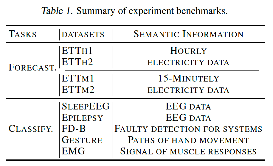
a) Benchmakrs

9 real-world datasets

b) Baslines

5 SSL pretraining methods

• TF-C (2022)
• TS-TCC (2021)
• Mixing-up (2022)

• TS2Vec (2022)

• TST (2021) … masked modeling methods

To demonstrate the generality of SimMTM…

also apply 3 advanced TS models as encoder

• (1) NSTransformer (2022) … SOTA model
• (2) Autoformer (2021)
• (3) Vanilla Transformer (2017)

Encoder

• default encoder : Vanilla Transformer

• for the classification : 1D-ResNet

c) Implementations

fine-tuning performance

• under both in- and cross-domain settings.

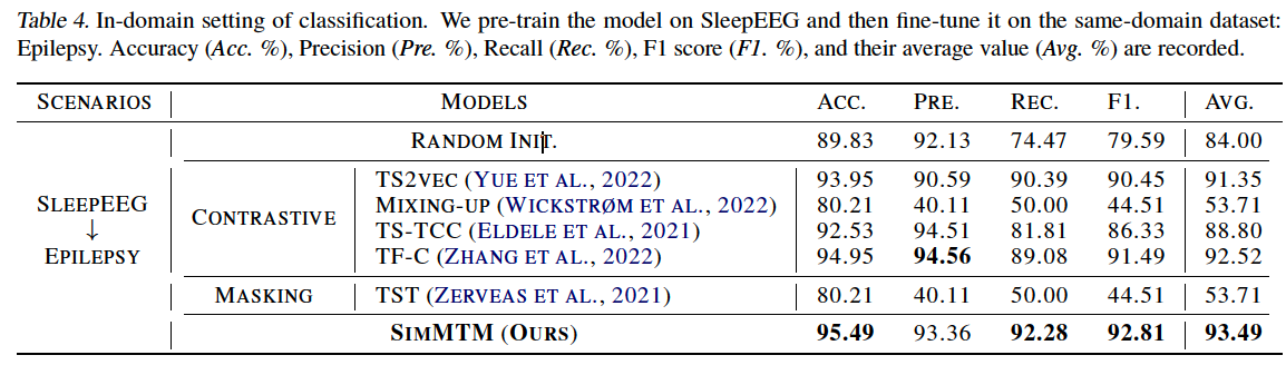
In-domain

• pre-train and fine-tune the model using the same or same-domain dataset

• ex) classification

  • SleepEEG & Epilepsy : quite similar semantic information

    ( denote as SleepEEG \(\rightarrow\) Epilepsy )

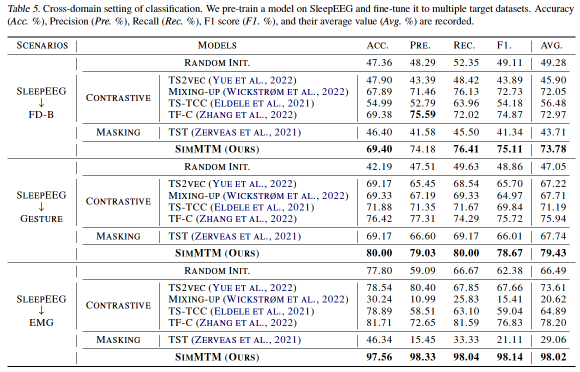
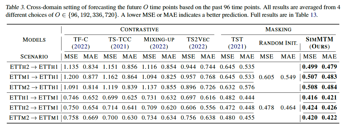
Cross-domain

• pre-train the model on a certain dataset
• fine-tune the encoder to different datasets.

(2) Main Results

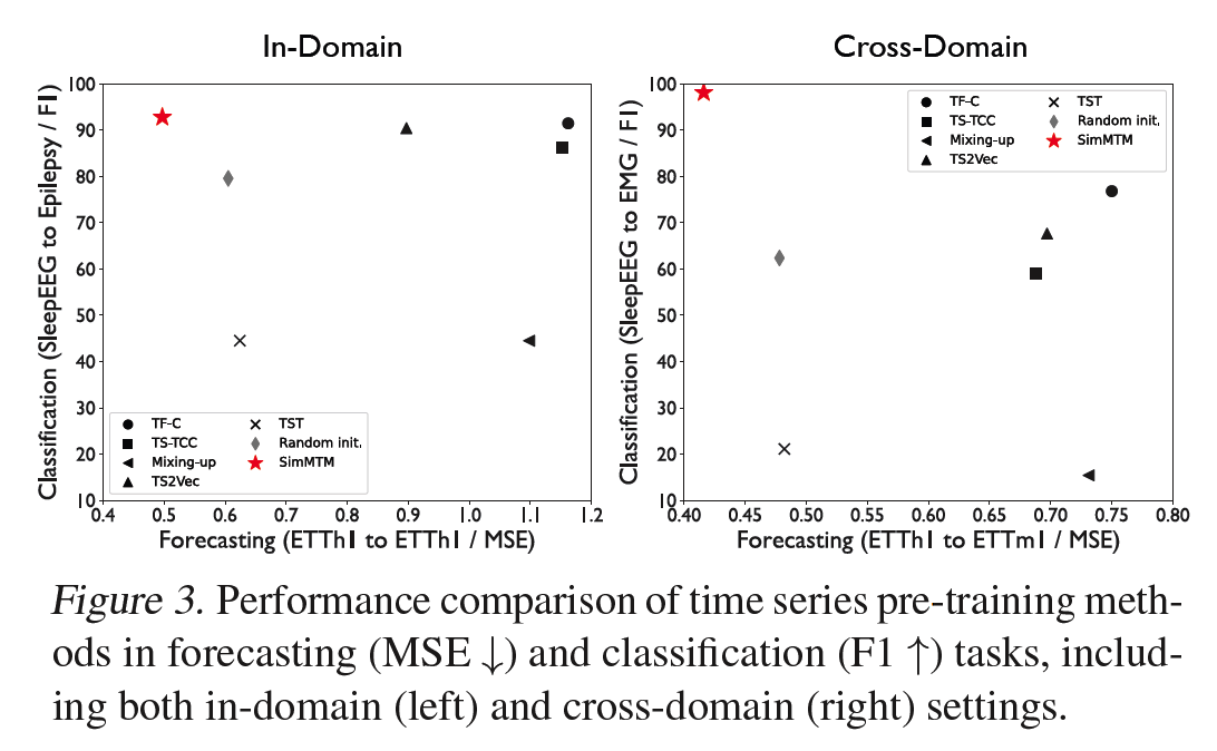
(masking-based method) TST (2021)

• forecasting task : GOOD
• classification task : BAD

CL methods

• forecasting task : BAD
• classification task : GOOD

Previous methods cannot cover both the “high-level” and “low-level” tasks simultaneously, highlighting the advantages of SimMTM in task generality

(3) Forecasting

outperforms, regardless of

• (1) masking-based methods
• (2) CL-based methods

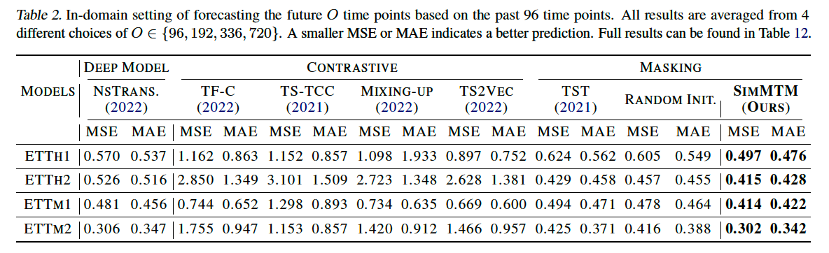
(masking-based) TST outperforms all CL methods

• directly adopts vanilla masking protocol into TS
• indiciates that “masked modeling” based on “point-wise reconstruction” is well suited for forecasting task ( than series-wise CL pretraining )

(4) Classification