VAE + GMM

Deep Unsupervised Clustering with Gaussian Mixture Gaussian Mixture VAE

Contents

1. Abstract
2. Introduction
3. GMVAE
   1. Generative & Recognition models
   2. Inference with the Recognition Model
   3. KL cost of the Discrete Latent Variable
   4. Over-regularization problem

0. Abstract

variant of VAE with GMM as prior

• goal : unsupervised clustering via DGM

Problem of regular VAE : over-regularisation

\(\rightarrow\) leads to cluster degeneracy

Minimum information constraint

• mitigate these problems in VAE
• improve unsupervised clustering performance

1. Introduction

Unsupervised clustering

• (conventional) K-means, GMM

  • limitation : similarity measures are limited to local relations in the data space

• DGM (Deep Generative Model)

  • can encode rich latent structures

  • can be used for dimensionality reduction

  • try to estimate the density of observed data under some assumptions

    ( assumption about about its latent structure )

    \(\rightarrow\) They allow us to reason about data in more complex ways

  • ex) VAE

Proposal :

• perform unsupervised clustering within VAE

• over-regularisation in VAEs

  \(\rightarrow\) can be mitigated with the minimum information constraint

2. GMVAE

( Gaussian Mixture Variational Auto Encoder )

Vanilla VAE vs GM-VAE

• (Vanilla VAE) prior : isotropic Gaussian
  • interpretable, but unimodal ….
• (GM-VAE) prior : mixture of Gaussian

variational lower bound of our GMVAE can be optimised with standard back-prop

( through the reparametrisation trick )

(1) Generative & Recognition models

[ Generative model ]

\[p_{\beta, \theta}(\boldsymbol{y}, \boldsymbol{x}, \boldsymbol{w}, \boldsymbol{z})=p(\boldsymbol{w}) p(\boldsymbol{z}) p_\beta(\boldsymbol{x} \mid \boldsymbol{w}, \boldsymbol{z}) p_\theta(\boldsymbol{y} \mid \boldsymbol{x})\]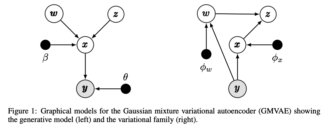

\(\boldsymbol{y} \mid \boldsymbol{x} \sim \mathcal{N}\left(\boldsymbol{\mu}(\boldsymbol{x} ; \theta), \operatorname{diag}\left(\boldsymbol{\sigma}^2(\boldsymbol{x} ; \theta)\right)\right) \text { or } \mathcal{B}(\boldsymbol{\mu}(\boldsymbol{x} ; \theta))\).

• \(\boldsymbol{x} \mid z, \boldsymbol{w} \sim \prod_{k=1}^K \mathcal{N}\left(\boldsymbol{\mu}_{z_k}(\boldsymbol{w} ; \beta), \operatorname{diag}\left(\boldsymbol{\sigma}_{z_k}^2(\boldsymbol{w} ; \beta)\right)\right)^{z_k}\).
  • \(\boldsymbol{w} \sim \mathcal{N}(0, \boldsymbol{I})\).
  • \(z \sim \operatorname{Mult}(\boldsymbol{\pi})\).
    • set the parameter \(\pi_k=K^{-1}\) to make \(\mathbf{z}\) uniformly distributed
• \(K\) : pre-defined number of components

Model ( NN ) : \(\boldsymbol{\mu}_{z_k}(\cdot ; \beta), \boldsymbol{\sigma}_{z_k}^2(\cdot ; \beta), \boldsymbol{\mu}(\cdot ; \theta), \boldsymbol{\sigma}^2(\cdot ; \theta)\).

(2) Inference with the Recognition Model

Loss function : ELBO

• \(\mathcal{L}_{E L B O}=\mathbb{E}_q\left[\frac{p_{\beta, \theta}(\boldsymbol{y}, \boldsymbol{x}, \boldsymbol{w}, \boldsymbol{z})}{q(\boldsymbol{x}, \boldsymbol{w}, \boldsymbol{z} \mid \boldsymbol{y})}\right]\),

MFVI (Mean-Field Variational Inference)

assume the mean-field variational family \(q(\boldsymbol{x}, \boldsymbol{w}, \boldsymbol{z} \mid \boldsymbol{y})\) as a proxy to posterior

factorization :

• \(q(\boldsymbol{x}, \boldsymbol{w}, \boldsymbol{z} \mid \boldsymbol{y})=\prod_i q_{\phi_x}\left(\boldsymbol{x}_i \mid \boldsymbol{y}_i\right) q_{\phi_w}\left(\boldsymbol{w}_i \mid \boldsymbol{y}_i\right) p_\beta\left(\boldsymbol{z}_i \mid \boldsymbol{x}_i, \boldsymbol{w}_i\right)\).
  • \(i\) : index of data point …. but drop for convenience

parametrise each variational factor with the recognition networks

• recognition networks : \(\phi_x\) and \(\phi_w\)
  • output : params of the variational distns

\(p_\beta(\boldsymbol{z} \mid x, \boldsymbol{w})\) ( \(z\)-posterior )

• \(\begin{aligned} p_\beta\left(z_j=1 \mid \boldsymbol{x}, \boldsymbol{w}\right) &=\frac{p\left(z_j=1\right) p\left(\boldsymbol{x} \mid z_j=1, \boldsymbol{w}\right)}{\sum_{k=1}^K p\left(z_k=1\right) p\left(\boldsymbol{x} \mid z_j=1, \boldsymbol{w}\right)} \\ &=\frac{\pi_j \mathcal{N}\left(\boldsymbol{x} \mid \mu_j(\boldsymbol{w} ; \beta), \sigma_j(\boldsymbol{w} ; \beta)\right)}{\sum_{k=1}^K \pi_k \mathcal{N}\left(\boldsymbol{x} \mid \mu_k(\boldsymbol{w} ; \beta), \sigma_k(\boldsymbol{w} ; \beta)\right)} \end{aligned}\).

Rewrite ELBO

\(\begin{aligned} \mathcal{L}_{E L B O}=& \mathbb{E}_{q(\boldsymbol{x} \mid \boldsymbol{y})}\left[\log p_\theta(\boldsymbol{y} \mid \boldsymbol{x})\right]-\mathbb{E}_{q(\boldsymbol{w} \mid \boldsymbol{y}) p(\boldsymbol{z} \mid \boldsymbol{x}, \boldsymbol{w})}\left[K L\left(q_{\phi_x}(\boldsymbol{x} \mid \boldsymbol{y}) \mid \mid p_\beta(\boldsymbol{x} \mid \boldsymbol{w}, \boldsymbol{z})\right)\right] \\ &-K L\left(q_{\phi_w}(\boldsymbol{w} \mid \boldsymbol{y}) \mid \mid p(\boldsymbol{w})\right)-\mathbb{E}_{q(\boldsymbol{x} \mid \boldsymbol{y}) q(\boldsymbol{w} \mid \boldsymbol{y})}\left[K L\left(p_\beta(\boldsymbol{z} \mid \boldsymbol{x}, \boldsymbol{w}) \mid \mid p(\boldsymbol{z})\right)\right] \end{aligned}\).

• \(\mathbb{E}_{q(\boldsymbol{x} \mid \boldsymbol{y})}\left[\log p_\theta(\boldsymbol{y} \mid \boldsymbol{x})\right]\) : reconstruction term
• \(\mathbb{E}_{q(\boldsymbol{w} \mid \boldsymbol{y}) p(\boldsymbol{z} \mid \boldsymbol{x}, \boldsymbol{w})}\left[K L\left(q_{\phi_x}(\boldsymbol{x} \mid \boldsymbol{y}) \mid \mid p_\beta(\boldsymbol{x} \mid \boldsymbol{w}, \boldsymbol{z})\right)\right]\) : conditional prior term
• \(K L\left(q_{\phi_w}(\boldsymbol{w} \mid \boldsymbol{y}) \mid \mid p(\boldsymbol{w})\right)\) : \(w\)-prior
• \(\mathbb{E}_{q(\boldsymbol{x} \mid \boldsymbol{y}) q(\boldsymbol{w} \mid \boldsymbol{y})}\left[K L\left(p_\beta(\boldsymbol{z} \mid \boldsymbol{x}, \boldsymbol{w}) \mid \mid p(\boldsymbol{z})\right)\right]\) :\(z\)-prior

a) reconstruction term

estimated by drawing Monte Carlo samples from \(q(\boldsymbol{x} \mid \boldsymbol{y})\)

• ( + back-prop using reparameterization trick )

b) Conditional Prior term

\(\begin{gathered} \mathbb{E}_{q(\boldsymbol{w} \mid \boldsymbol{y}) p(\boldsymbol{z} \mid \boldsymbol{x}, \boldsymbol{w})}\left[K L\left(q_{\phi_x}(\boldsymbol{x} \mid \boldsymbol{y}) \mid \mid p_\beta(\boldsymbol{x} \mid \boldsymbol{w}, \boldsymbol{z})\right)\right] \approx \\ \frac{1}{M} \sum_{j=1}^M \sum_{k=1}^K p_\beta\left(z_k=1 \mid \boldsymbol{x}^{(j)}, \boldsymbol{w}^{(j)}\right) K L\left(q_{\phi_x}(\boldsymbol{x} \mid \boldsymbol{y}) \mid \mid p_\beta\left(\boldsymbol{x} \mid \boldsymbol{w}^{(j)}, z_k=1\right)\right) \end{gathered}\).

• no need to sample from the discrete distribution \(p(z \mid \boldsymbol{x}, \boldsymbol{w})\).
• \(p_\beta(\boldsymbol{z} \mid \boldsymbol{x}, \boldsymbol{w})\) : can be computed with one forward pass
• expectation of \(q_{\phi_w}(\boldsymbol{w} \mid \boldsymbol{y})\) : can be estimated with \(M\) samples

c) \(w\)-prior term

calculated analytically

d) \(z\)-prior term

• in (3)

(3) KL cost of the Discrete Latent Variable

reduce the KL divergence between the \(z\)-posterior & uniform prior

• by concurrently manipulating the position of the clusters and the encoded point \(x\)

\(\rightarrow\) merge the clusters by maximising the overlap between them, and moving the means closer together

(4) Over-regularizaiton problem

Result of strong influence of the prior

\(\rightarrow\) problem : overly simplified

This problem is still prevalent in the assignment of the GMVAE

2 main approaches to overcome this effect:

• (1) anneal the KL term

  • during training by allowing the reconstruction term to train the AE,

    before slowly incorporating the regularization from the KL term

• (2) modify the objective function

  • by setting a cut-off value that removes the effect of the KL term,

    when it is below a certain threshold