
Predictive Temporal Embedding of Dynamic Graphs (2020)
Contents
-
Abstract
-
Introduction
-
Related Work
- Static Graph
- Dynamic Graphs
-
Problem Definition
- Dynamic Graph
- Graph History
- Graph Embedding
-
Preliminaries & Notation
- GNN
- GGNN
-
Recurrent Models for Dynamic Graphs
-
Dynamic Graph Autoencoder
- DyGrAE
- Temporal Message Propagation
- Temporal Encoder
-
Temporal Decoder
- Objective Function
-
Dynamic Graph Predictor
- DyGrPr
- Temporal Attention
- Temporal Decoder
- Objective Function
-
Training
-
0. Abstract
Previous works : static graph
Representation Learning for the entire graph in a dynamic context is yet to be addressed
\(\rightarrow\) propose an UNsupervised enc-dec framework, that projects a DYNAMIC graph at each time step into \(d\)-dim space
2 different strategies
- (1) address representation learning proble, by auto-encoding the graph dynamics
- (2) formulate a graph prediction problem & enforce the encoder to learn the representation, that an autoregressive decoder uses to predict the future
Model : uses (1) GGNNs + (2) LSTM
1. Introduction
Dynamic graph :
-
edges change over time
nodes can appear/disappear over time
-
often defined as time-ordered sequences of network snapshots
Graph Representation Learning
- many processes over dynamic graphs depend on the temporal dynamics ( not just topology of connections )
- ideal approach : should be able to learn both
Propose an..
- (1) UNsupervised learning approach
- (2) for DYNAMIC graph representaiton
- (3) that combines the power of STATIC graph representation & RNN
Model
- seq2seq framework
- 2 strategies
- (1) modify encoder-decoder paradigm, to propose a dynamic graph autoencoder
- use GGNN in encoder
- reconstruct using autoregressive decoder
- (2) formulate a dynamic graph prediction task
- (1) modify encoder-decoder paradigm, to propose a dynamic graph autoencoder
2. Problem Definition
(1) Dynamic Graph
Definition : ordered sequence of \(T\) graph snapshots
-
\(G=\left\langle G_{1}, G_{2}, \ldots, G_{T}\right\rangle\),
where \(G_{t}=\left(V_{t}, E_{t}\right)\) models the state of a dynamic system at the interval \([t, t+\Delta t]\)
Dynamic graph \(G\)
- Subset of nodes from the set \(V\) at each time step, \(V_{t} \subset V\).
- Each node \(v \in V_{t}\) takes a unique identification
- Edges : \(e_{k j}^{t} \in E_{t}\) : pair of nodes \((k, j) \in\) \(\left\{E_{t}: V_{t} \times V_{t}\right\}\)
- Adjacency matrix : \(A_{t} \in \mathbb{R}^{n \times n}\)
(2) Graph History
\(H_{G_{t}}=\left\langle G_{t-w}, G_{t-w+1}, G_{t-w+2}, \ldots, G_{t-1}\right\rangle\).
(3) Graph Embedding
Given \(H_{G_{t}}\), seek to learnn mapping function
4. Preliminaries & Notation
(1) GGNN
Summary of GGNN
-
extension of GNNs
-
to learn the reachability across the nodes in a graph.
-
use GRU to propagate a message from a node to all its reachable nodes
This paper : define the propagation model in GGNNs
Notation
- \(A\) : adjacency matrix
- \(x_{v} \in \mathbb{R}^{k}\) : initial node embedding ( drawn from uniform distn )
- \(n_{i}^{v}\) : hidden state of node \(v\) at iteration \(i\)
Propagation : \(a_{i}^{v}=A_{v:}\left[n_{i-1}^{1} \ldots n_{i-1}^{ \mid V \mid }\right]+b\)
- run several iterations
Node state: \(n_{i}^{v}=\left(1-z_{i}^{v}\right) \odot n_{i-1}^{v}+z_{i}^{v} \odot \widetilde{n}_{i}^{v}\)
5. Recurrent Models for Dynamic Graphs
-
GGNN’s ability to capture topology of graph
-
LSTM enc-dec to capture dynamics of the graph
Decoder
- reconstructs the dynamics, observed by the encoder
Encoder
-
autoencoders for dynamic graphs
\(\rightarrow\) called Dynamic Graph AutoEncoder ( = DyGrAE )
-
Then, explore the dynamic graph representaiton learning,
- by encoding the dynamics of graph history &
- by predicting its future dynamics
\(\rightarrow\) called Dynamic Graph Predictor ( = DyGrPr )
(1) Dynamic Graph Autoencoder
a) DyGrAE
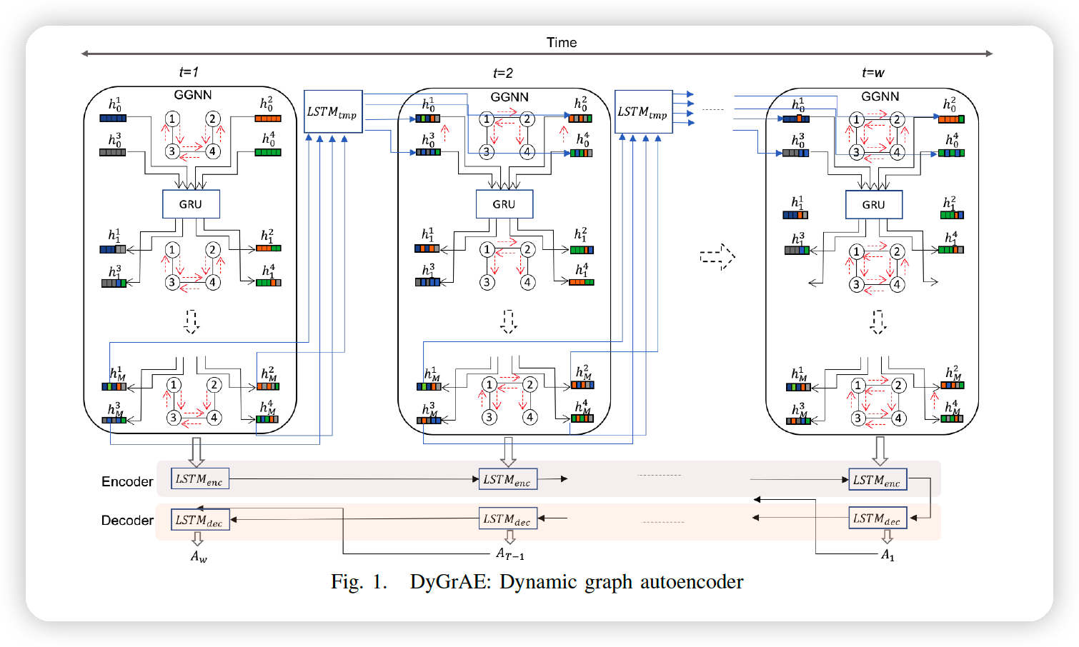
4 main components
- (1) GGNN : to capture topology of the graph at \(t\)
- (2) RNN : to propagate temporal information across time steps
- (3) encoder : to project the graph evolution over a window of \(w\) into \(d\) dim
- (4) decoder : to reconstruct the structure of dynamic graph
a-1) GGNN
-
build a graph representation for \(G_T\)
-
After \(M\) step of message propagation,
use an average pooling of nodes’ hidden states
\(\operatorname{Emb}_{G G N N}\left(G_{t}\right)=\operatorname{Avg}\left(n_{M}^{v}\right)\).
a-2) Temporal Message Propagation
-
to deal with dynamic connectivity and reachability among nodes across different time steps
-
temporal path
-
a sequence of edges: \(L=\left\langle e_{i j}^{l 1}, e_{j k}^{l 2}, \cdots, e_{m n}^{l n}\right\rangle\)
-
node \(u\) is directly reachable from node \(v\) at time step \(t\) ,
if there exists an edge \(u v\) at timestep \(t\), i.e., \(a_{v u}^{t}=1\).
-
-
Propagate messages,
- not only in the topology of the graph at each time step
- but also during a temporal window of graph evolution
\(\rightarrow\) add a temporal message propagation module using LSTM
Model
- \(\operatorname{NodesInit}\left(G_{t}\right)=L S T M_{t m p}\left(G G N N_{t-1}, h_{t-1}^{t m p}\right)\).
- \[G G N N_{t-1}=\left\{n_{M}^{v}(t-1) \mid v \in V\right\}\]
a-3) Temporal Encoder
\(h_{t}^{e n c}=L S T M_{e n c}\left(\operatorname{Emb}_{G G N N}\left(G_{t}\right), h_{t-1}^{e n c}\right)\).
a-4) Temporal Decoder
\(h_{t}^{\text {dec }}=L S T M_{d e c}\left(\bar{A}^{t-1}, h_{t-1}^{d e c}\right)\).
Objective Function
parameter space of the models :
-
includes parameters related to \(G G N N\), \(L S T M_{e n c}\), \(L S T M_{d e c}, L S T M_{t m p}\), \(W \in \mathbb{R}^{ \mid h^{d e c} \mid \times \mid V \mid ^{2}}\) and \(b \in \mathbb{R}^{ \mid V \mid ^{2}}\).
-
use cross entropy loss
\(\operatorname{Loss}_{C E}= \left.-\sum_{o \in O} \sum_{t=1}^{w} \sum_{i=1}^{ \mid V \mid } \sum_{j=1}^{ \mid V \mid } A_{i j}^{t} \log \left(\bar{A}_{i j}^{t}\right)\right)+\left(1-A_{i j}^{t}\right) \log \left(1-\bar{A}_{i j}^{t}\right)\).
(2) Dynamic Graph Predictor
we focus on representation learning by enforcing encoder to learn the representation such that the decoder can predict the future evolution of the graph
a) DyGrPr
Graph history vector = context vector, that summarizes history of the graph
( The architectures of GGNN, temporal message propagation and temporal encoder, remain the same as DyGrAE )
b) Temporal Attention
-
takes into account the evolution of graph, observed by the temporal encoder
( in order to predict the evolution of graph in the future )
-
forces the model to focus on the time steps that have SIGNIFICANT IMPACT on governing the future evolution of a dynamic graph
\(\begin{array}{r} \alpha_{t}^{i}=f\left(h_{t-1}^{d e c}, h_{i}^{e n c}\right) \in \mathbb{R} \\ \overline{\alpha_{t}}=\operatorname{softmax}\left(\alpha_{t}\right) \\ h_{t}^{*}=\sum_{i=t-w}^{t-1} \bar{\alpha}_{t}^{i} \cdot h_{i}^{e n c} \end{array}\).
c) Temporal Decoder
\(h_{t}^{d e c}=L S T M_{d e c}\left(\left[h_{t}^{*}, \bar{A}^{t-1}\right], h_{t-1}^{d e c}\right)\).
d) Objective Function
same as above