TabDDPM; Modeling Tabular Data with Diffusion Models

TabDDPM: Modeling Tabular Data with Diffusion Models

Contents

1. Abstract
2. Related Work
3. Background
4. TabDDPM
5. Experiments

0. Abstract

Diffusion models can be advantageous for general tabular problems

Tabular data = vectors of heterogeneous features

( Some are discrete / continuous )

\(\rightarrow\) Makes it quite challenging for accurate modeling

TabDDPM

• Diffusion model that can be universally applied to any tabular dataset
• Handles any type of featur
• Superiority over existing GAN/VAE alternatives
• Eligible for privacy-oriented setups

https://github.com/rotot0/tab-ddpm.

1. Related Work

(1) Diffusion models

• pass

(2) Generative models for tabular problems

• High-quality synthetic data is of large demand for many tabular tasks

• (1) Tabular datasets are often limited in size

• (2) Proper synthetic datasets do not contain actual user data

  \(\rightarrow\) Can be publicly shared without violation of anonymity

Recent works

• Tabular VAEs (Xu et al., 2019)
• GAN-based approaches (Xu et al., 2019; Engelmann & Lessmann, 2021; Jordon et al., 2018; Fan et al., 2020; Torfi et al., 2022; Zhao et al., 2021; Kim et al., 2021; Zhang et al., 2021; Nock & Guillame-Bert, 2022; Wen et al., 2022).

(3) “Shallow” synthetics generation

Tabular data is typically structured

• Individual features are often interpretable
• Not clear if their modelling requires several layers of “deep” architectures

\(\rightarrow\) Simple interpolation techniques, like SMOTE (Chawla et al., 2002) can serve as simple and powerful solutions

3. Background

(1) Gaussian diffusion

Operate in continuous spaces \(\left(x_t \in \mathbb{R}^n\right)\)

Forward process

• \(q\left(x_t \mid x_{t-1}\right):=\mathcal{N}\left(x_t ; \sqrt{1-\beta_t} x_{t-1}, \beta_t I\right)\).

• \(q\left(x_T\right):=\mathcal{N}\left(x_T ; 0, I\right)\).

Reverse process

• \(p_\theta\left(x_{t-1} \mid x_t\right):=\mathcal{N}\left(x_{t-1} ; \mu_\theta\left(x_t, t\right), \Sigma_\theta\left(x_t, t\right)\right)\).

DDPM

• Using diagonal \(\Sigma_\theta\left(x_t, t\right)\) with a constant \(\sigma_t\)
• Computing \(\mu_\theta\left(x_t, t\right)\) as a function of \(x_t\) and \(\epsilon_\theta\left(x_t, t\right)\)
  • \(\mu_\theta\left(x_t, t\right)=\frac{1}{\sqrt{\alpha_t}}\left(x_t-\frac{\beta_t}{\sqrt{1-\bar{\alpha}_t}} \epsilon_\theta\left(x_t, t\right)\right)\).
  • where \(\alpha_t:=1-\beta_t, \bar{\alpha}_t:=\prod_{i \leq t} \alpha_i\)
• Loss function: \(L_t^{\text {simple }}=\mathbb{E}_{x_0, \epsilon, t} \mid \mid \epsilon-\epsilon_\theta\left(x_t, t\right) \mid \mid _2^2\).

(2) Multinomial diffusion

To generate categorical data

• where \(x_t \in\{0,1\}^K\) is a one-hot encoded categorical variable with \(K\) values.

Forward process

• \(q\left(x_t \mid x_{t-1}\right)\) : categorical distribution that corrupts the data by uniform noise over \(K\) classes
• \(q\left(x_t \mid x_{t-1}\right):=\operatorname{Cat}\left(x_t ;\left(1-\beta_t\right) x_{t-1}+\beta_t / K\right)\).
• \(q\left(x_T\right):=\operatorname{Cat}\left(x_T ; 1 / K\right)\).

• \(q\left(x_t \mid x_0\right)=\operatorname{Cat}\left(x_t ; \bar{\alpha}_t x_0+\left(1-\bar{\alpha}_t\right) / K\right)\).

• \(q\left(x_{t-1} \mid x_t, x_0\right)=C a t\left(x_{t-1} ; \pi / \sum_{k=1}^K \pi_k\right)\).
  • where \(\pi=\left[\alpha_t x_t+\left(1-\alpha_t\right) / K\right] \odot\left[\bar{\alpha}_{t-1} x_0+\left(1-\bar{\alpha}_{t-1}\right) / K\right]\).

Reverse process

• \(p_\theta\left(x_{t-1} \mid x_t\right)\) is parameterized as \(q\left(x_{t-1} \mid x_t, \hat{x}_0\left(x_t, t\right)\right)\),
  • where \(\hat{x}_0\) is predicted by NN

4. TabDDPM

(1) Data

Categorical & Numerical features

• [Categorical and Binary] Multinomial diffusion
• [Numerical] Gaussian diffusion

Tabular data sample \(x=\left[x_{\text {num }}, x_{\text {cat }_1}, \ldots, x_{\text {cat }_C}\right]\),

• \(N_{\text {num }}\) numerical features \(x_{\text {num }} \in \mathbb{R}^{N_{\text {num }}}\)
  • takes normalized numerical features
• \(C\) categorical features \(x_{\text {cat }_i}\) with \(K_i\) categories each
  • takes one-hot encoded versions of categorical features as an input (i.e. \(x_{\text {cat }_i}^{\text {ohe }} \in\{0,1\}^{K_i}\) )

\(\rightarrow\) Input \(x_0\) has a dimensionality of \(\left(N_{n u m}+\sum K_i\right)\).

(2) Preprocessing

[REG] Gaussian quantile transformation

[CLS] Handled by a separate forward diffusion process ( = independently )

Reverse diffusion step in TabDDPM is modelled by a MLP

& output of the same dimensionality as \(x_0\),

• where the first \(N_{n u m}\) coordinates are the predictions of \(\epsilon\) for the Gaussian diffusion and the rest are the predictions of \(x_{\text {cat }_i}^{\text {ohe }}\) for the multinomial diffusions.

(3) Losses

Two losses

• (1) MSE \(L_t^{\text {simple }}\) for the Gaussian diffusion term

• (2) KL divergences \(L_t^i\) for each multinomial diffusion term

\(\rightarrow\) \(L_t^{T a b D D P M}=L_t^{\text {simple }}+\frac{\sum_{i \leq C} L_t^i}{C}\).

(4) Cls. vs. Reg.

Classification/Regression datasets

• [CLS] Class conditional model, i.e. \(p_\theta\left(x_{t-1} \mid x_t, y\right)\)
• [REG] Consider a target value as an additional numerical feature, and the joint distribution is learned

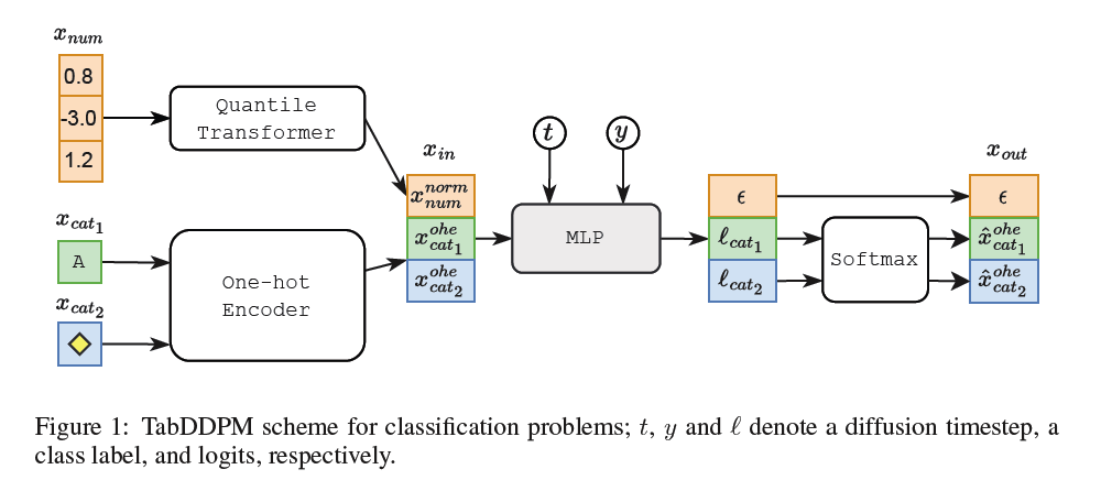
(5) Architectures

Architectures

\(\begin{aligned} & \operatorname{MLP}(x)=\text { Linear }(\operatorname{MLPBlock}(\ldots(\operatorname{MLPBlock}(x)))) \\ & \operatorname{MLPBlock}(x)=\operatorname{Dropout}(\operatorname{ReLU}(\operatorname{Linear}(x))) \end{aligned}\).

For a tabular input \(x_{i n}\), a timestep \(t\), and a class label \(y\) ….

\(\begin{aligned} & t_{-} e m b=\text { Linear }(\text { SiLU }(\text { Linear }(\operatorname{SinTimeEmb~}(t)))) \\ & y \_e m b=\text { Embedding }(y) \\ & x=\text { Linear }\left(x_{i n}\right)+t \_e m b+y \_e m b \end{aligned}\).

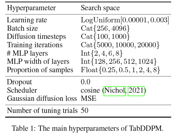
(6) Hyperparameters

5. Experiments

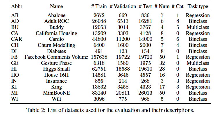
(1) Settings

a) Datasets

b) Baselines

( Only the baselines with the published source code )

1. TVAE (Xu et al., 2019)
   • SOTA VAE for tabular data generation
2. CTABGAN (Zhao et al., 2021)
   • Recent GAN-based model that is shown to outperform the existing tabular GANs
   • Cannot handle regression tasks.
3. CTABGAN+(Zhao et al., 2022)
   • Extension of the CTABGAN model
4. SMOTE (Chawla et al., 2002)
   • “Shallow” interpolation-based method that ”generates” a synthetic point as a convex combination of a real data point and its k-th nearest neighbor from the dataset.
   • Originally proposed for minor class oversampling.

c) Evaluation Measure

ML efficiency (or utilizty)

• Quantifies the performance of CLS or REG models,

  • which are trained on synthetic data and
  • evaluated on real test set

• Use 2 evaluation protoco;ls to compute ML efficiency

  • (1) Average efficiency w.r.t a set of diverse ML models

  • (2) ML efficiency only w.r.t CatBoost model ( = leading GBDT )

    \(\rightarrow\) (2) is more crucial than (1)

d) Tuning process

Tuning process is guided by …

• The values of the ML efficiency (with respect to Catboost)

  of the generated synthetic data

  on a hold-out validation dataset (the score is averaged over five different sampling seeds).

• Search spaces for all hyperparameters : Table 1

Demonstrate that

• Tuning the hyperparameters using the CatBoost guidance does not introduce any sort of “Catboost-biasedness”
• Catboost-tuned TabDDPM produces synthetics that are also superior for other models, like MLP.

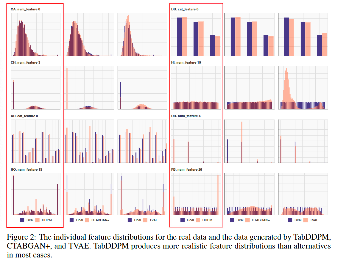
(1) Qualitative Comparison

Sample a synthetic dataset from TabDDPM, TVAE, and CTABGAN+ of the same size as a real train set

• (for CLS datasets) Each class is sampled according to its proportion in the real dataset

Visualize the typical individual feature distributions for real and synthetic data : Figure 2.

• Result) TabDDPM produces more realistic feature distributions

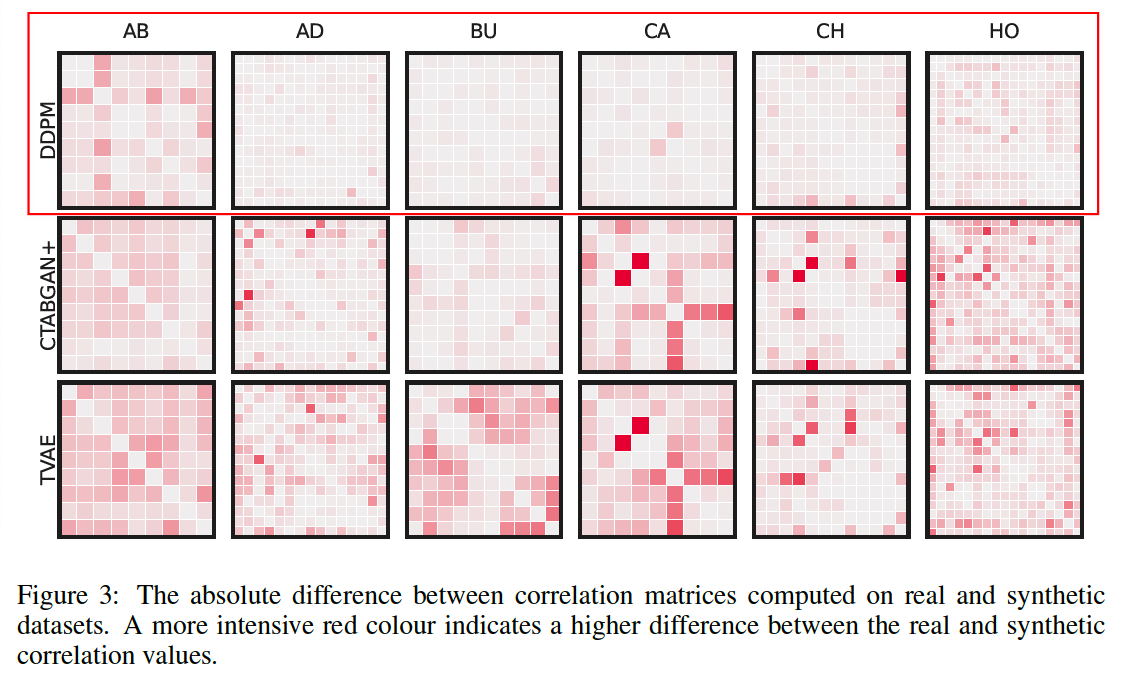
Visualize the differences between the correlation matrices computed on real vs. synthetic data

• Pearson correlation coefficient: for numerical-numerical correlations

• correlation Ratio: for categorical-numerical cases
• Theil’s U statistic: between categorical features

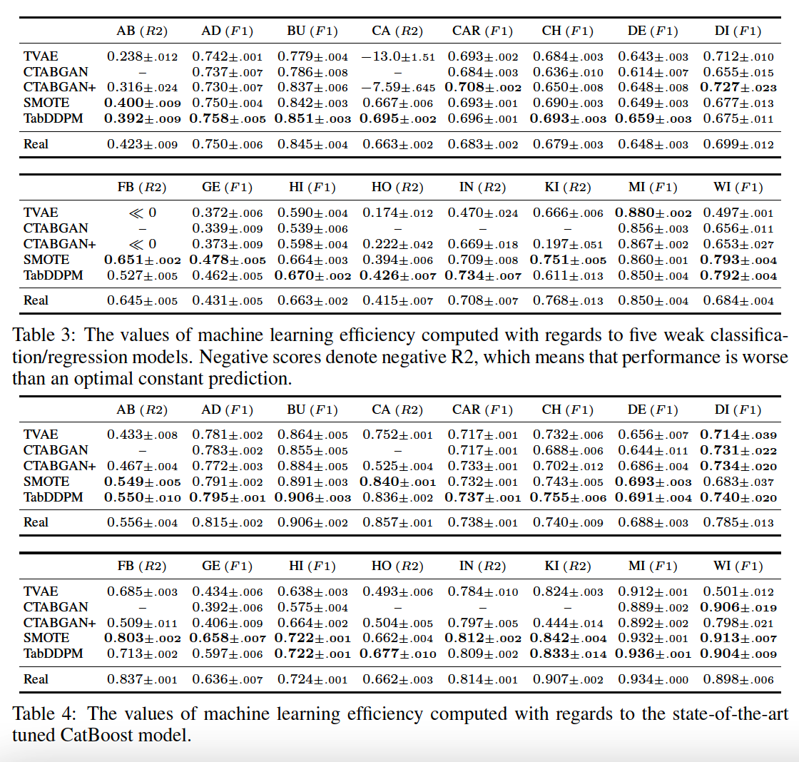
(2) ML Efficiency

a) Metric

• Classification : F1 score
• Reression : R2 score

b) Two protocols

1. Average ML efficiency for a diverse set of ML models

   • ex) Decision Tree, Random Forest, Logistic Regression (or Ridge Regression) and MLP models

2. ML efficiency w.r.t the SOTA model for tabular data

   • ex) CatBoost and MLP architecture

     • hyperparameters are thoroughly tuned on each dataset using the search spaces from (Gorishniy et al., 2021).

   • This protocol demonstrates the practical value of synthetic data more reliably

     ( \(\because\) In most real scenarios practitioners are not interested in using weak and suboptimal classifiers/regressors )

c) Main results.