STASY; Score-based Tabular Data Synthesis

STASY: Score-based Tabular Data Synthesis

Contents

1. Abstract

2. Introduction

3. Related Work

4. Proposed Method

   1. Score Network & Miscellaneous Designs
   2. Self-paced Learning
   3. Fine-tuning Approach

0. Abstract

Score-based Tabular data Synthesis (STaSy)

Training Strategy

• “Self-paced learning” technique
• “Fine-tuning strategy” which further increases the sampling quality and diversity
  • by stabilizing the denoising score matching training

1. Introduction

Previous works

• CTGAN (Xu et al., 2019), TVAE (Xu et al. , 2019), IT-GAN (Lee et al., 2021), and OCT-GAN (Kim et al., 2021).
• Score-based generative modeling (SGMs)

Score-based Tabular data Synthesis (STaSy)

• Adopt a score-based generative modeling paradigm
• Outperform all existing baselines in terms of the sampling quality and diversity

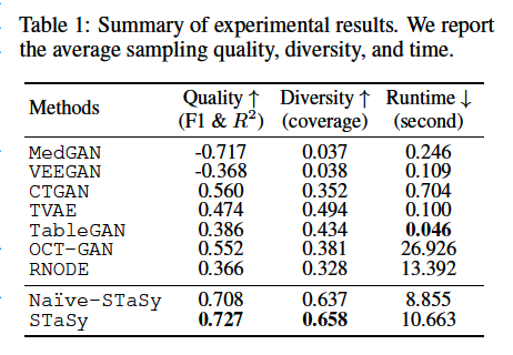
• Naive-STaSy: naive conversion of SGMs toward tabular data
• STaSy: Naive-STaSy + proposed self-paced learning and fine-tuning methods

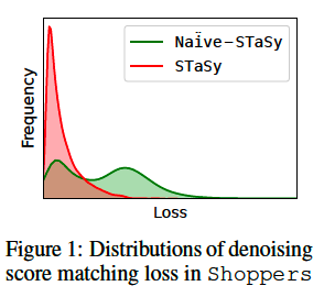
• Naive-STaSy

  • Uneven and long-tailed loss distribution at the end of its training process

  • Failed to learn the score values of some records.

    \(\rightarrow\) (partially) underfitted to training data.

• STaSy

  • Two proposed training methods
  • Yields many loss values around the left corner

Training strategies

1. Self-paced learning method

   • Trains our model from “easy to hard” records

     ( based on their loss values by modifying the objective function )

   • Makes the model learn records selectively and eventually

2. Fine-tuning approach

   • Further improve the sampling quality and diversity.

Contributions

1. Design a score-based generative model for tabular data synthesis
2. Alleviate the training difficulty of the denoising score matching loss by …
   • (1) Self-paced learning strategy
   • (2) Enhance the sampling quality and diversity using a proposed fine-tuning method
3. Outperforms other deep learning methods in all cases by large margins

2. Related Work

(1) Score-based Generative models

SDE: \(d \mathbf{x}=\mathbf{f}(\mathbf{x}, t) d t+g(t) d \mathbf{w}\).

Depending on the types of \(f\) and \(g\)…

• SGMs can be divided into
  • variance exploding (VE)
  • variance preserving (VP)
  • sub-variance preserving (sub-VP)

Reverse of the diffusion process

• \(d \mathbf{x}=\left(\mathbf{f}(\mathbf{x}, t)-g^2(t) \nabla_{\mathbf{x}} \log p_t(\mathbf{x})\right) d t+g(t) d \mathbf{w}\).
• Score function \(\nabla_{\mathbf{x}} \log p_t(\mathbf{x})\) is approximated by a score network \(S_{\boldsymbol{\theta}}(\mathrm{x}, t)\),

Train a score network \(S_{\boldsymbol{\theta}}(\mathrm{x}, t)\) as …

• \(\underset{\boldsymbol{\theta}}{\arg \min } \mathbb{E}_t \mathbb{E}_{\mathbf{x}(t)} \mathbb{E}_{\mathbf{x}(0)}\left[\lambda(t) \mid \mid S_{\boldsymbol{\theta}}(\mathbf{x}(t), t)-\nabla_{\mathbf{x}(t)} \log p(\mathbf{x}(t) \mid \mathbf{x}(0)) \mid \mid _2^2\right]\).

Sampling

• (1) Predictor-corrector framework
• (2) Probability flow method
  • a deterministic method based on the ODE
  • the latter enables fast sampling and exact log-probability computation.

(2) Tabular Data Synthesis

Recursive table modeling utilizing a Gaussian copula is used to synthesize continuous variables (Patki et al., 2016).

Discrete variables can be generated by Bayesian networks (Zhang et al., 2017; Aviñó et al., 2018) and decision trees (Reiter, 2005).

Several data synthesis methods based on GANs

• RGAN (Esteban et al., 2017): creates continuous time-series healthcare records
• MedGAN (Choi et al., 2017) and corrGAN (Patel et al., 2018): generate discrete records
• EhrGAN (Che et al., 2017): utilizes semi-supervised learning
• PATE-GAN (Jordon et al. 2019): generates synthetic data without jeopardizing the privacy of real data.
• TableGAN (Park et al., 2018): employs CNN to enhance tabular data synthesis and maximize label column prediction accuracy.
• CTGAN and TVAE (Xu et al., 2019): adopt column-type-specific preprocessing steps to deal with multi-modality in the original dataset distribution.
• OCT-GAN (Kim et al., 2021): generative model design based on neural ODEs.
• SOS (Kim et al., 2022): style-transfer-based oversampling method for imbalanced tabular data using SGMs, whose main strategy is converting a major sample to a minor sample.

(3) Self-Paced Learning

“Curriculum learning”

= select training records in a meaningful order

Training a model only with a subset of data ,

that has LOW training losses & gradually expanding to the *training data**.

Notation

• Training set \(\mathcal{D}=\left\{\mathbf{x}_i\right\}_{i=1}^N\), where \(\mathbf{x}_i\) is the \(i\)-th record
• Model \(M\) with parameters \(\theta\)
• Loss \(l_i=L\left(M\left(\mathrm{x}_i, \boldsymbol{\theta}\right)\right)\),
• Vector \(\mathrm{v}=\left[v_i\right]_{i=1}^N, v_i \in\{0,1\}\) indicates whether \(\mathrm{x}_i\) is easy or not for all \(i\).

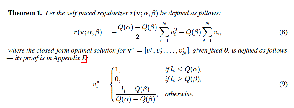
SPL aims to learn the (1) model parameter \(\theta\) and the (2) selection importance \(\mathrm{v}\) by minimizing:

• \(\min _{\boldsymbol{\theta}, \mathbf{v}} \mathbb{E}(\boldsymbol{\theta}, \mathbf{v})=\sum_{i=1}^N v_i L\left(M\left(\mathbf{x}_i, \boldsymbol{\theta}\right)\right)-\frac{1}{K} \sum_{i=1}^N v_i\).
  • where \(K\) is a parameter to control the learning pace.
• Second term: self-paced regularizer
  • Can be customized for a downstream task.

“Alternative convex search (ACS)”

( Used to solve above Equation )

• Alternately optimizing variables while fixing others

  ( i.e., update \(\mathrm{v}\) after fixing \(\theta\), and vice versa )

• With fixed \(\theta\), the global optimum \(\mathbf{v}^*=\left[v_i^*\right]_{i=1}^N\) is defined as …

  • \(v_i^*= \begin{cases}1, & l_i<\frac{1}{K}, \\ 0, & l_i \geq \frac{1}{K},\end{cases}\).

Record \(\mathrm{x}_i\) with \(l_i<\frac{1}{K}\) = Easy record = Chosen for training

To involve more records in the training process, \(K\) is gradually decreased.

3. Proposed Method

• (1) SPL: for training stability
• (3) Fine-tuning method takes advantage of a favorable property of SGMs, which is that we can measure the log-probabilities of records

(1) Score Network & Miscellaneous Designs

This to consider!!

• (1) Each column in tabular data typically has complicated distributions
• (2) Tabular synthesis models should learn the joint probability of multiple columns
• (3) One good design point is that the dimensionality of tabular data is typically far less than that of image data
  • ex) 784 pixels even in MNIST
  • ex) 30 columns in Credit.

Proposed score network architecture

• Consists of residual blocks of FC layers
• \(T=50\) steps in Equation 1 are enough to train a network
  • naturally has less sampling time than SGMs for images

Pre/post-processing of tabular data

To handle mixed types of data, pre/post-process columns.

• [NUM] Min-max scaler
  • Reverse scaler is used for post-processing after generation
• [CAT] One-hot encoding
  • Softmax function when generating.

Sampling

• Step 1) Sample noisy vector \(\mathrm{z} \sim \mathcal{N}\left(\mu, \sigma^2 \mathbf{I}\right)\)
  • varies depending on the type of SDEs: \(\mathcal{N}\left(\mathbf{0}, \sigma_{\max }^2 \mathrm{I}\right)\) for \(\mathrm{VE}\), and \(\mathcal{N}(\mathbf{0}, \mathbf{I})\) for \(\mathrm{VP}\) and sub-VP
• Step 2) Reverse SDE can convert \(\mathrm{z}\) into a fake record
  • Adopt the probability flow method to solve the reverse SDE

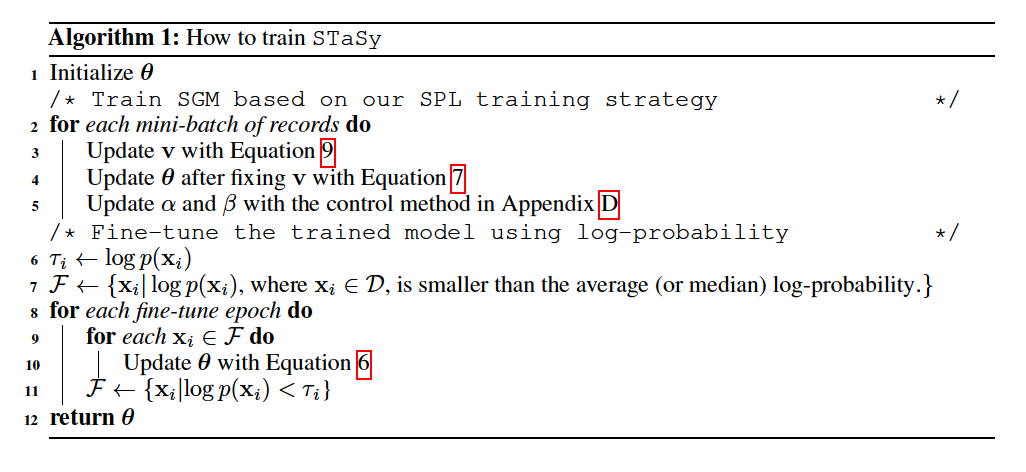
(2) Self-paced Learning

Apply a curriculum learning technique

“Soft” record sampling

• instead of \(v_i \in\{0,1\}\),
• use \(v_i \in[0,1]\).

Denoising score matching loss for \(\mathbf{x}_i\) :

• \(l_i=\mathbb{E}_t \mathbb{E}_{\mathbf{x}_i(t)}\left[\lambda(t) \mid \mid S_{\boldsymbol{\theta}}\left(\mathbf{x}_i(t), t\right)-\nabla_{\mathbf{x}_i(t)} \log p\left(\mathbf{x}_i(t) \mid \mathbf{x}_i(0)\right) \mid \mid _2^2\right]\).

STaSy loss function:

• \(\min _{\boldsymbol{\theta}, \mathbf{v}} \sum_{i=1}^N v_i l_i+r(\mathbf{v} ; \alpha, \beta)\).
  • where \(0 \leq v_i \leq 1\) for all \(i\)
  • \(r(\cdot)\) is a self-paced regularizer.
  • \(\alpha \in[0,1]\) and \(\beta \in[0,1]\) are variables to define thresholds

(3) Fine-tuning Approach

Reverse SDE process

• With the approximated score function \(S_{\boldsymbol{\theta}}(\cdot)\),
• the probability flow method uses the following neural ODE
  • \(d \mathbf{x}=\left(\mathbf{f}(\mathbf{x}, t)-\frac{1}{2} g(t)^2 \nabla_{\mathbf{x}} \log p_t(\mathbf{x})\right) d t\).

\(\rightarrow\) Able to calculate the exact log-probability efficiently

\(\rightarrow\) Propose to fine-tune based on the exact log-probability.