PatchTST Experiments
Contents
- SL
- SSL
- TL
- Comparison with other SSL
- Ablation Study
- Patching & CI
- Varying $L$
- Varying $P$
- Model Parameters
- Visualization
- Channel-Independence Analysis
1. SL
(1) Datasets
8 datasets for LTSF
- large dataset : weather, traffic, electricity
- small dataset : ILI + 4 ETT datasets
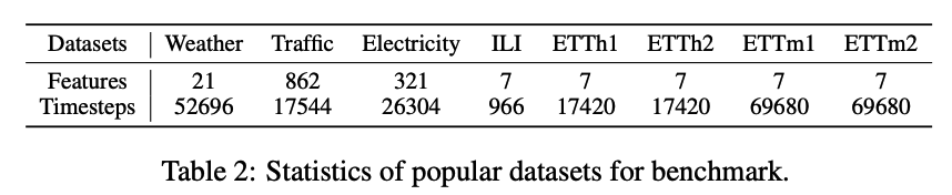
Descriptions
-
Weather : 21 meteorogical indicators ( ex. humidity, air temperature … )
-
Traffic : road occupancy rates from different sensors
-
Electricity : 321 customers’ hourly electricity consumption
-
ILI : number of patients & influenza-like illness ratio ( weekly )
-
ETT ( Electricity Transformer Temperature ) : collected from 2 different elecgtiricy transformers
-
ETTm : 15 mintues
-
ETTh : 1 hour
-
Etc ) Exchange-rate
- daily exchange-rate of 8 countirers
- financial datasets : different properties
- Ex) last-value prediction = BEST result
(2) Baseline Settings
Prediction Length :
- ILI : [24,36,48,60]
- others : [96,192,336,720]
Lookback Window ( except for ILI ) :
- DLinear : 336
- xx-former : ( original : 96 )
- because if LONG… prone to OVERFITTING
- thus, rerun in [24,48,96,..720] & chose the best one for stronger baseline
Lookback Window for ILI:
- DLinear : 36
- xx-former : ( original : 104)
- because if LONG… prone to OVERFITTING
- thus, rerun in [24,36,48,60,104,144] & chose the best one for stronger baseline
(3) Model Variants
2 versions of PatchTST
- PatchTST/64
- number of patches = 64
- lookback window = 512
- patch length = 16
- stride = 8
- PatchTST/42
- number of patches = 42
- lookback window = 336
- patch length = 16
- stride = 8
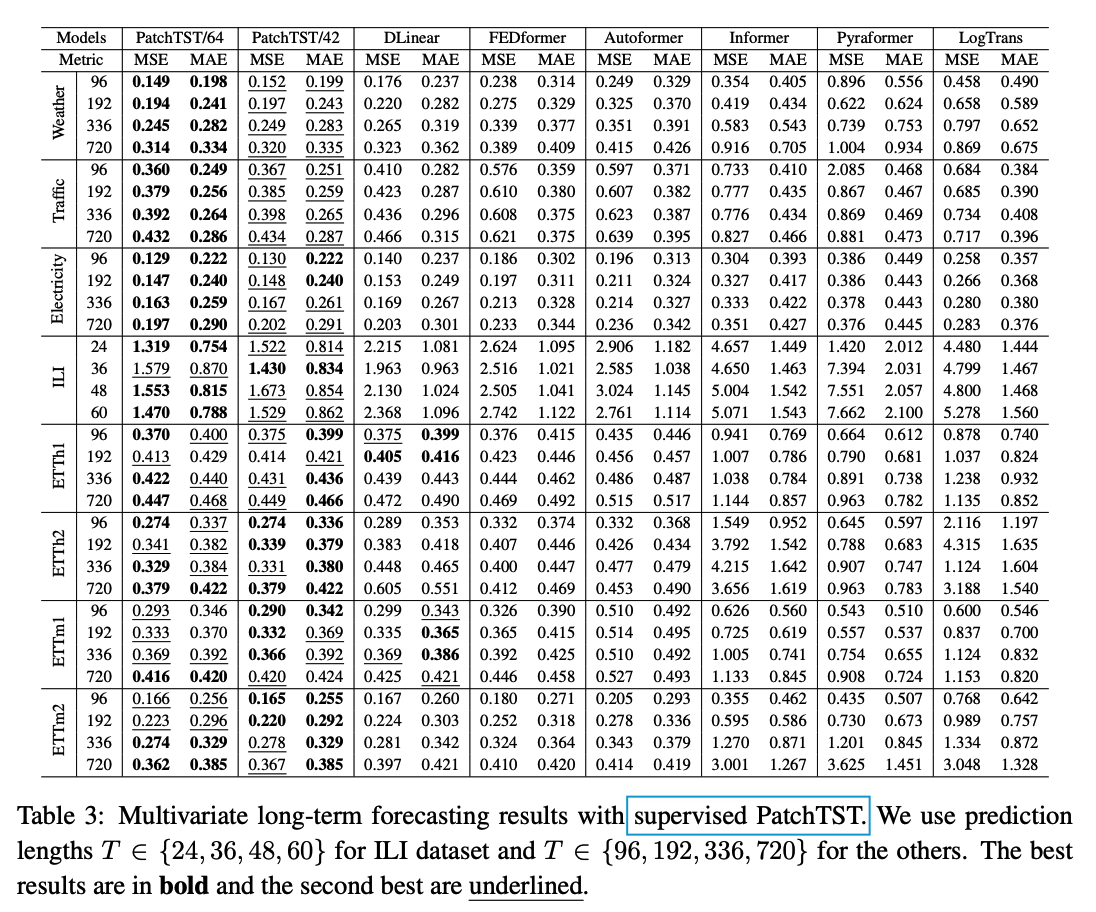
(4) Results
( Compared with DLinear )
- outperform especially in LARGE datasets ( Weather, Traffic, Electricity) & ILI
2. SSL
Details
- NON-overlapped patch
- masking ratio : 40% ( with zero )
Input settings
- input size = 512
- number of patches = 42
- patch length & stride = 12
Procedure
- step 1) Pretraining 100 epochs
- step 2)
- 2-1) Linear Probing ( 20 epochs )
- 2-2) E2E fine-tuning ( linear probing 10 epochs + E2E 20 epochs )
Results
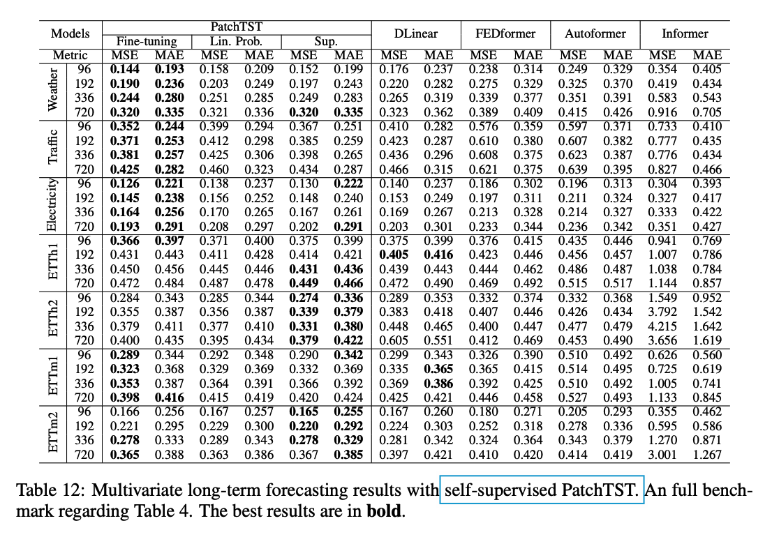
- Fine-tuning > Linear Probing = Supervised
Large datasets ( Weather, Traffic, Electricity )
- Fine-tuning > Supervised >= Linear Probing
Middle datasets ( Ettm1, Ettm2 )
- Fine-tuning = Supervised >= Linear Probing
Small datasets ( others except Ettm1 )
- Supervised > Fine-tuning = Linear Probing
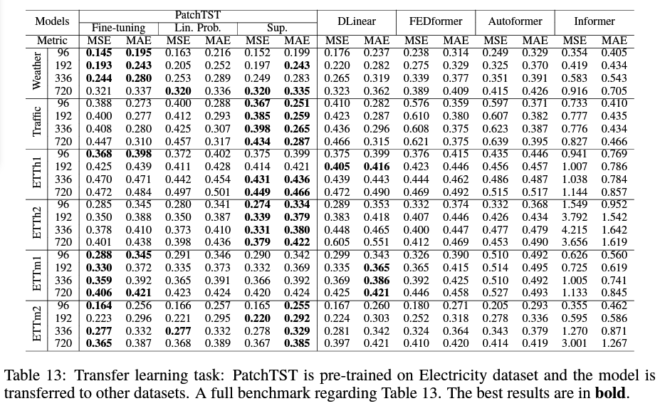
3. TL
Source dataset : Electricity
Target dataset : others
4. Comparison with other SSL
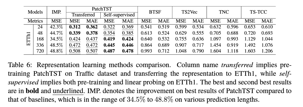
-
for fair comparison, do Linear-Probing
-
2 versions
- Transfered : ( source = Electricity )
- SSL
5. Ablation Study
(1) Patching & Channel Independence
Patching
-
improves running time & memory consumption
( due to shorter input )
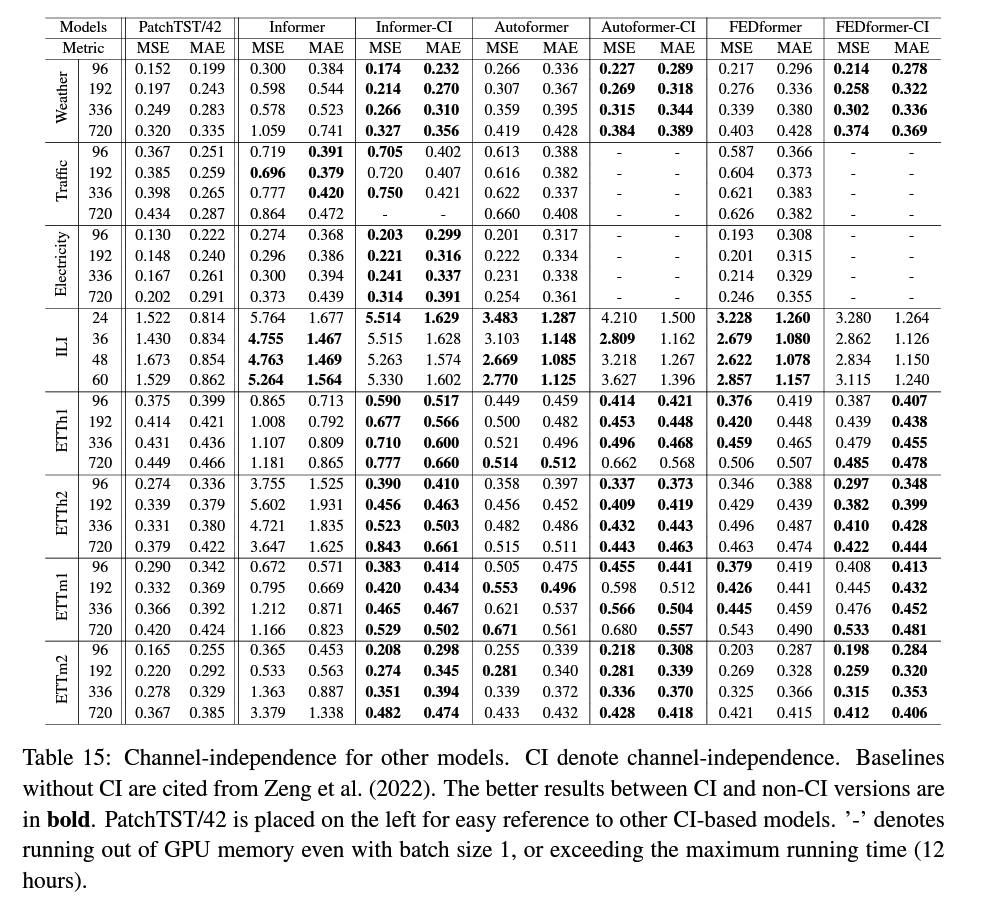
Channel Independence
- Not intuitive
- In-depth analysis
Patching & CI
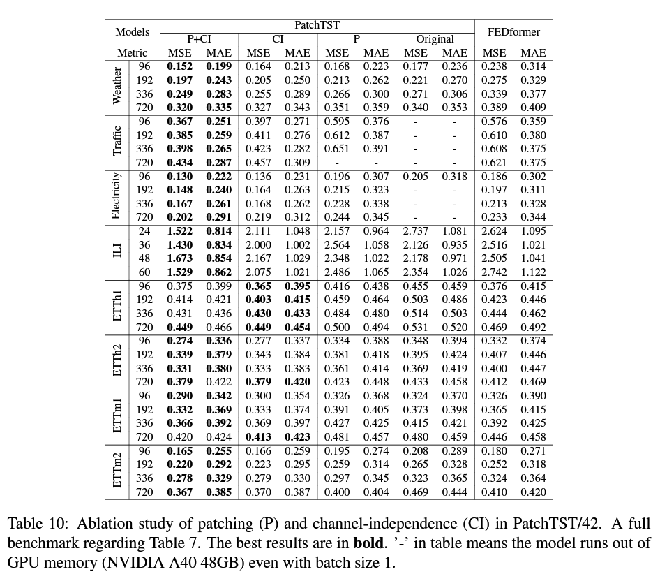
Deeper into CI
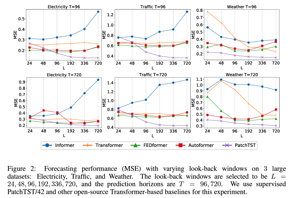
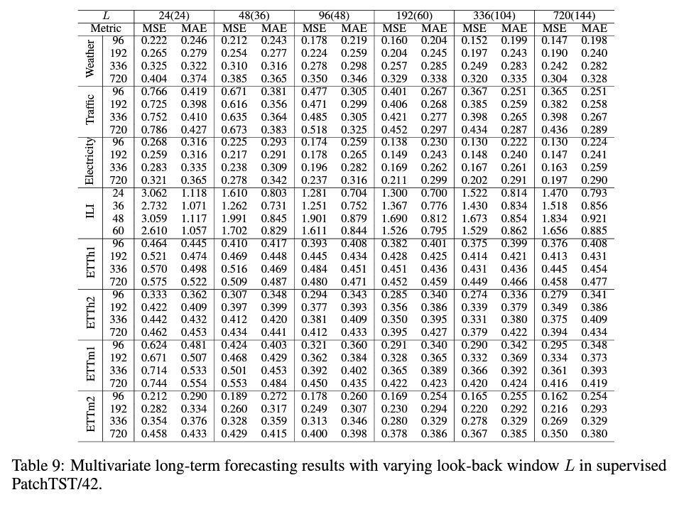
(2) Varying Look-back Window
( Transfomer ) the longer \(\rightarrow\) the better (X)
( PatchTST ) the longer \(\rightarrow\) the better (O)
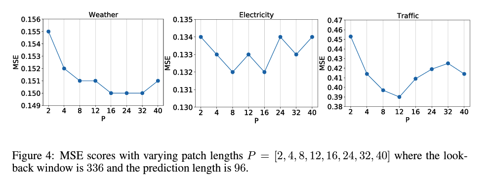
(3) Varying Patch Length
Lookback window = 336
Patch size = [4, 8, 16, 24, 32, 40]
- stride = patch size ( no overlapping )
Goal : predict 96 steps
Result : ROBUST to \(P\)
6. Model Parameters
3 encoder layers
- number of head : H
- dim of latent space : D
- dim of new latent space : F
activation function : GELU
dropout : 0.2
Architecture ( H - D - F)
- (ILI, ETTh1, ETTh2) : ( 4 - 16 - 128 )
- (othersr) : ( 16 - 128 - 256 )
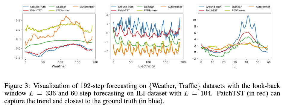
7. Visualization
8. Channel-Independence Analysis
Channel-mixing
- input token takes the vector of all TS features & projects it to embedding space to mix information
Channel-independence
- means that each input token only contains information from a single channel.
Intuition ) Channel-Mixing > Channel-Independence
( \(\because\) flexiblity to explore cross-channel information )
Why CI > CM ?
3 key factors
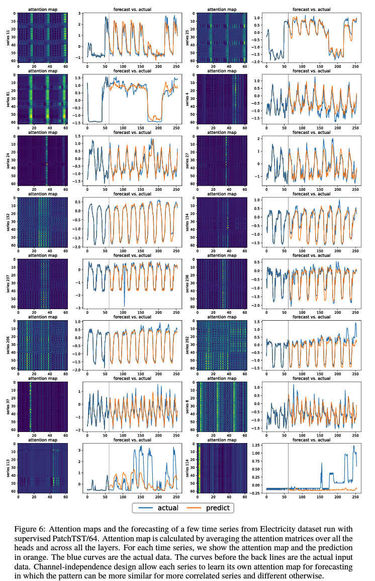
- (1) Adaptability ( Figure 6 )
- CI : different patterns for different series
- CM : all the series share the same attention patterns
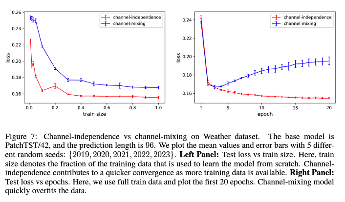
- (2) CM need more training data
- may need more data to learn information from different channels & different time steps jointly
- CI converges faster than CM
- (3) Overfitting : CM > CI ( Figure 7 )