11.(EM algorithm) EM algorithm (2)

3. EM Algorithm (2)

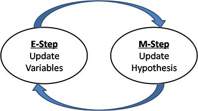
We have seen that EM algorithm consists of two parts.

https://stillbreeze.github.io/images/em.jpg

• E-step : fix \(\theta\), maximize the lower bound with respect to \(q\)
  
  

• M-step : fix \(q\), maximize the lower bound with respect to \(\theta\)
  
  

Let’s talk about each step more in detail.

(1) E-step (Expectation)

It tries to maximize the lower bound with respect to \(q\) ( while fixing \(\theta\) ). That is same as minimizing the “gap between lower bound and log likelihood”. The gap between these two can be expressed as a ‘KL-divergence’.
( use the same example(GMM with three mixtures) )

\[\begin{align*} GAP &= logp(X|\theta)-L(\theta,q) \\ &= \sum_{i=1}^{N}logp(X_i|\theta)-\sum_{i=1}^{N}\sum_{c=1}^{3}q(t_i=c)log\frac{p(X_i,t_i=c|\theta)}{q(t_i=c)}\\ &= \sum_{i=1}^{N}(logp(X_i|\theta)\sum_{c=1}^{3}q(t_i=c)-\sum_{c=1}^{3}q(t_i=c)log\frac{p(X_i,t_i=c|\theta)}{q(t_i=c)}\\ &=\sum_{i=1}^{N}\sum_{c=1}^{3}q(t_i=c)(logp(X_i|\theta)-log\frac{p(X_i,t_i=c|\theta)}{q(t_i=c)})\\ &=\sum_{i=1}^{N}\sum_{c=1}^{3}q(t_i=c)log\frac{p(X_i|\theta)q(t_i=c)}{p(X_i,t_i=c|\theta)} \\ &=\sum_{i=1}^{N}\sum_{c=1}^{3}q(t_i=c)log\frac{q(t_i=c)}{p(t_i=c|X_i,\theta)}\\ &=KL(q(t_i)||p(t_i=c \mid X_i,\theta))) \end{align*}\]

So, to maximize the lower bound, we minimize the KL-divergence. And to minimize the KL-divergence, we have to set \(q(t_i) = p(t_i = c \mid X_i,\theta)\)

General Expression :

(2) M-step (Maximization)

On M-step, we want to maximize this lower bound with respect to \(\theta\). It can be expressed as below.

( use the same example(GMM with three mixtures) )

As you can see, \(E_q\;log\;p(X,T\mid \theta)\) is (usually) a concave function with respect to theta, which is easy to optimize!

(3) Understanding EM-algorithm Visually

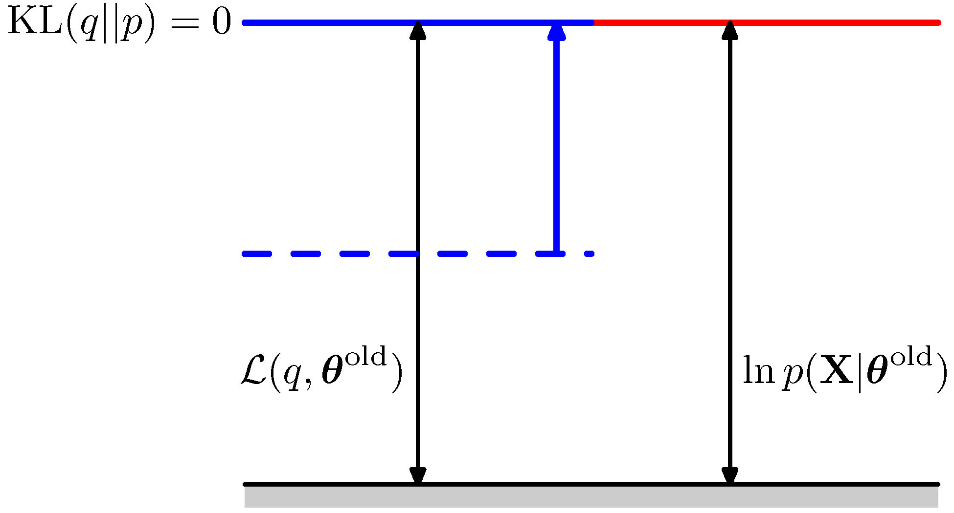
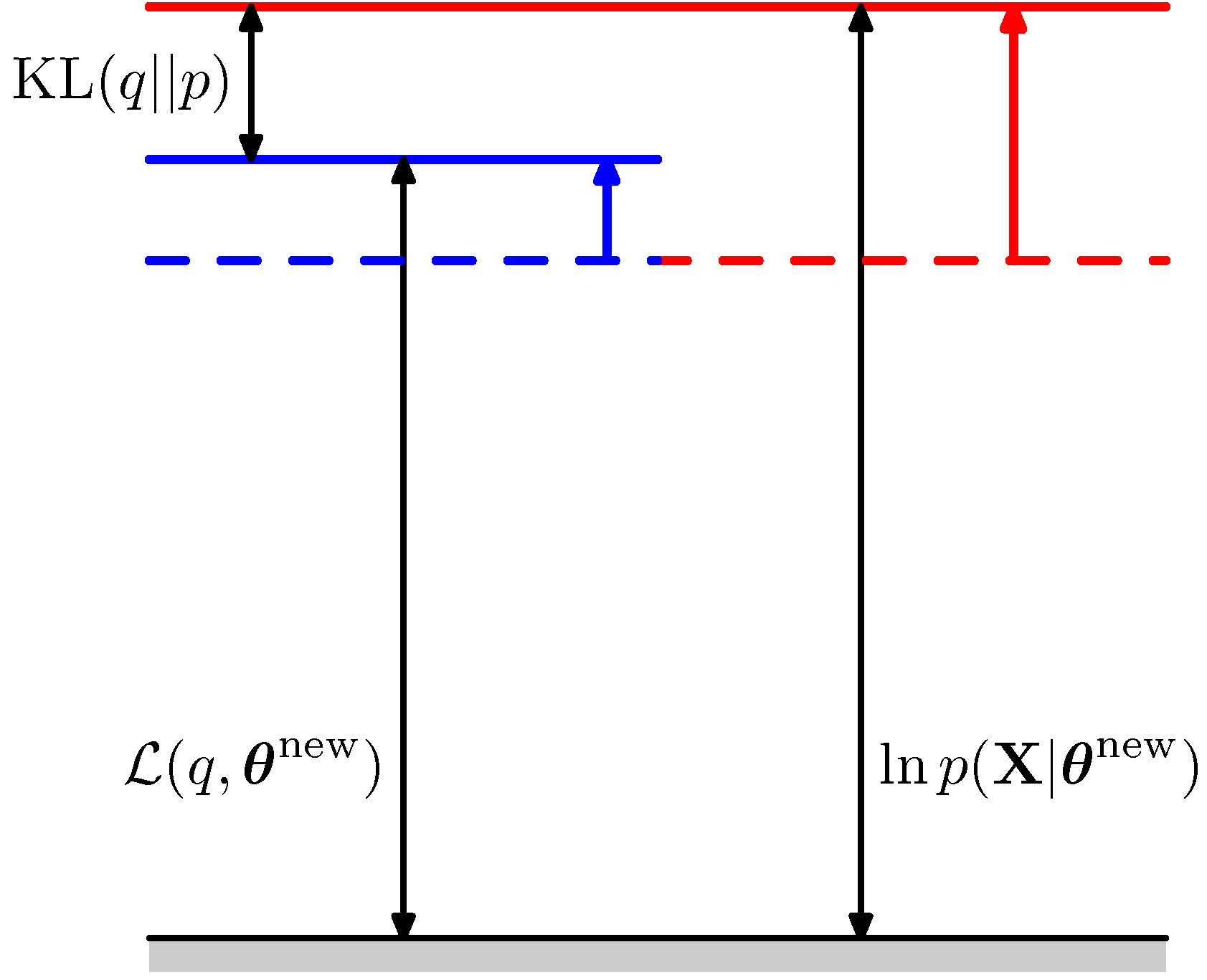
To write \(p\) in general form,


\(lnp(X|θ)=L(q,θ)+KL(q∥p)ln⁡p(X|θ)=L(q,θ)+KL(q‖p)\)

E step

• Make \(KL(q\mid \mid p)\) = 0, that is , pull up the blue line up to the red line!

</br>

M step

• fix \(q\) and find \(\theta^{new}\)
• that is, make the red line higher!

</br>

Repeat this E & M step!

(4) Summary of EM algorithm

[1] method for training Latent Variable Models

[2] Handles missing data

[3] sequence of simple tasks instead of one hard task

[4] guarantees to converge ( local or global )

[5] helps with complicated parameter constraints

[6] E & M step

In E-step, we maximize the lower bound with respect to q, and in the M-step, we maximize the lower bound with respect to theta. The mathematical expression will be like the below.

• E step :
  

• M step :