41.(paper 6) PPO (Proximal Policy Optimization)

( 참고 : Fastcampus 강의 )

[ 41. (paper 6) PPO (Proximal Policy Optimization) ]

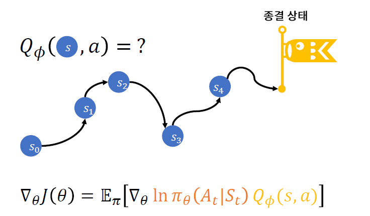
1. Actor-Critic의 불안정성

• 이유 1) 모든 \((s,a)\)를 방문하지 않을 수 있다. 방문하지 않은 \((s,a)\)에 대해서는 \(Q_{\phi}(s,a)\)의 추산이 부정확하다

• 이유 2) \(Q_{\phi}(s,a)\) 추산이 정확하다 하더라도, non-convex loss function으로 인한 local optimum에 빠질 수 있다

Solution : \(\pi_{\theta}\)가 급격히 바뀌지 않게끔 설계?

2. Background

PPO의 핵심 : (1) + (2)

• (1) Policy ( \(\pi_{\theta}\) ) 를 천천히 바꾸기
  • algorithm : CPI, TRPO
• (2) Advantage function을 정확히 추산하기
  • algorithm : GAE

(1) CPI & TRPO (Trust Region Policy Optimization)

• CPI : Conservative Policy Iteration

• TRPO : Trust Region Policy Optimization

  ( CPI의 가정 일부 완화 + 제약조건 )

Loss Function of CPI & TRPO

\(\max _{\theta} \widehat{\mathbb{E}}_{t}\left[\frac{\pi_{\theta}\left(a_{t} \mid s_{t}\right)}{\pi_{\theta_{o l d}}\left(a_{t} \mid s_{t}\right)} \hat{A}_{t}\right]\).

• CPI에서 제안한 loss function ( surrogate loss 라고도 부름 )

  ( policy의 old/new의 비율 x Advantage )

• 하지만 위의 목적함수를 단순히 optimize하면 너무 급격히 변할 수 있는 것을 우려하여…

• TRPO에서, 위에 “제약 조건 (constraint)”를 추가함

  such that \(\widehat{E}_{t}\left[K L\left[\pi_{\theta_{o l d}}\left(\cdot \mid s_{t}\right), \pi_{\theta}\left(\cdot \mid s_{t}\right)\right]\right] \leq \delta\).

Loss Function of PPO

두 policy의 비율 : \(r_{t}(\theta)=\frac{\pi_{\theta}\left(a_{t} \mid s_{t}\right)}{\pi_{\theta_{o l d}}\left(a_{t} \mid s_{t}\right)}\).

TRPO (CPI)의 objective function :

• \(L^{C P I}(\theta)=\widehat{\mathbb{E}}_{t}\left[\frac{\pi_{\theta}\left(a_{t} \mid s_{t}\right)}{\pi_{\theta_{\text {old }}}\left(a_{t} \mid s_{t}\right)} \hat{A}_{t}\right]=\widehat{\mathbb{E}}_{t}\left[r_{t}(\theta) \hat{A}_{t}\right]\).

PPO의 ojbective function :

• \(L^{C L I P}(\boldsymbol{\theta})=\widehat{\mathbb{E}}_{t}\left[\min \left(r_{t}(\theta) \hat{A}_{t}, \operatorname{clip}\left(r_{t}(\theta), 1-\epsilon, 1+\epsilon\right) \hat{A}_{t}\right)\right]\),

  where \(\operatorname{clip}\left(r_{t}(\theta), 1-\epsilon, 1+\epsilon\right)=\left\{\begin{array}{l} 1-\epsilon, r_{t}(\theta) \leq 1-\epsilon \\ 1+\epsilon, r_{t}(\theta) \geq 1+\epsilon\end{array}\right.\).

\(\rightarrow\) \(L^{C P I}(\theta) \geq L^{C L I P}\) … \(L^{C L I P}\) 가 더 보수적으로 update를 한다

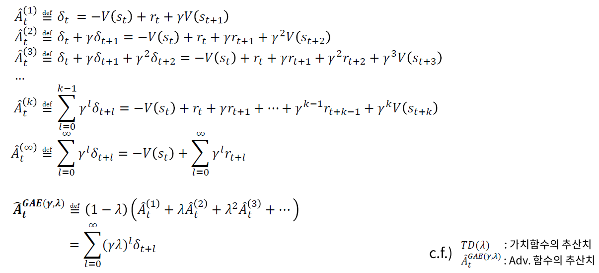
(2) Advantage Function : GAE

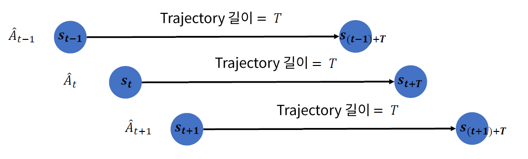
• 하지만 현실적으로 무한번 더할 수 없읍! use truncated version

• \(\hat{A}_{t}=\delta_{t}+(\gamma \lambda) \delta_{t+1}+\cdots+(\gamma \lambda)^{T-t+1} \delta_{T-1}\).

3. Loss Function of PPO

\[L_{t}^{C L I P+V F+S}(\theta)=\mathbb{E}_{t}\left[L_{t}^{C L I P}(\theta)-c_{1} L_{t}^{V F}(\theta)+c_{2} S\left[\pi_{\theta}\right]\left(s_{t}\right)\right]\]

• \(L_{t}^{V F}(\theta):\) Value Function Loss

  ( = \(V_{\theta}(s)\) 의 \(\theta\)를 최적화 )

• \(S\left[\pi_{\theta}\right]\left(s_{t}\right)\) = \(\mathcal{H}\left(\pi_{\theta}\left(a_{t} \mid s_{t}\right)\right)\)

4. PPO algorithm

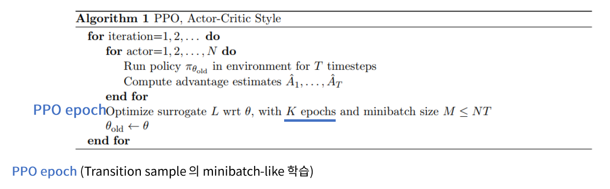
• 전체 샘플을 “한번에 update하지 않고”,

  “여러 번의 \(K\) epoch에 나눠서 update를 진행”

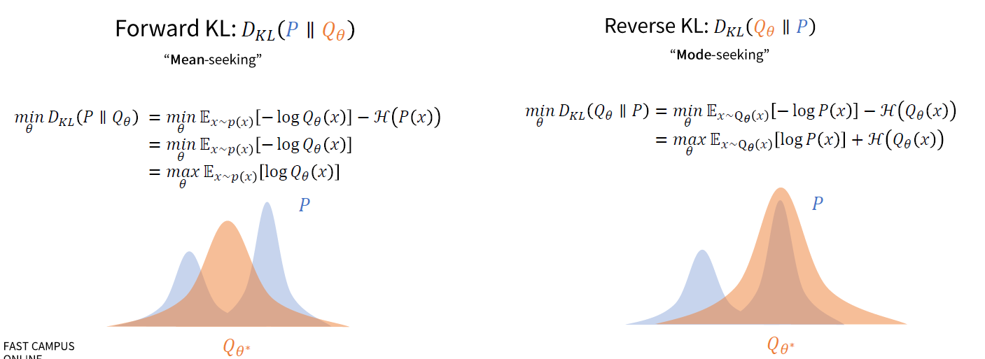
Appendix ) Forward & Backward KL-divergence