Diffusion-TS; Interpretable Diffusion for General Time Series Generation

Diffusion-TS: Interpretable Diffusion for General Time Series Generation

Contents

1. Abstract
2. Introduction
3. Problem Statement
4. Diffusion-TS: Interpretable Diffusion for TS
   1. Diffusion Framework
   2. Model Structure
   3. Fourier-based Training Objective
   4. Conditional Generation for TS Applications

Abstract

Diffusion-TS

• Geneate MTS
• 2 main characteristics
  • (1) Transformer-based method
  • (2) Disentangled temporal representations ( trend + seasonality + residual )
• Directly model the TS (instead of noise)
• Combine a Fourier-based loss term
• Easily extended to conditional generationt tasks ( imputation, forecasting)

1. Introduction

Diffusion model in TS

• most of them are task-specific generation (i.e. forecasting, imputation)
• some are unconditional: TSDiff (NeurIPS 2023)

Limitations

1. RNN: have limitation in long-range performance

2. No decomposition: w/o trend & seasonality

3. Not interpretable

Diffusion-TS

• Non-autoregressive diffusion model

• 2 key points
  • (1) Transformer-based architecture
  • (2) Disentangled seasonal-trend constitution of TS
• Design a Fourier-based loss … to reconstruct the “data” instead of “noise”

2. Problem Statement

Notation

• Dataset: \(D=\left\{X_{1: \tau}^i\right\}_{i=1}^N\)
• TS: \(X_{1: \tau}=\left(x_1, \ldots, x_\tau\right) \in \mathbb{R}^{\tau \times d}\)

Unconditional goal: use a diffusion-based generator to approach the function of \(\hat{X}_{1: \tau}^i=G\left(Z_i\right)\)

• which maps Gaussian vectors \(Z_i=\left(z_1^i, \ldots, z_t^i\right) \in \mathbb{R}^{\tau \times d \times T}\) to the signals
• \(T\) : total diffusion step

TS model with trend and multiple seasonality

• \(x_j=\zeta_j+\sum_{i=1}^m s_{i, j}+e_j, \quad j=0,1, \ldots, \tau-1\).

3. Diffusion-TS: Interpretable Diffusion for TS

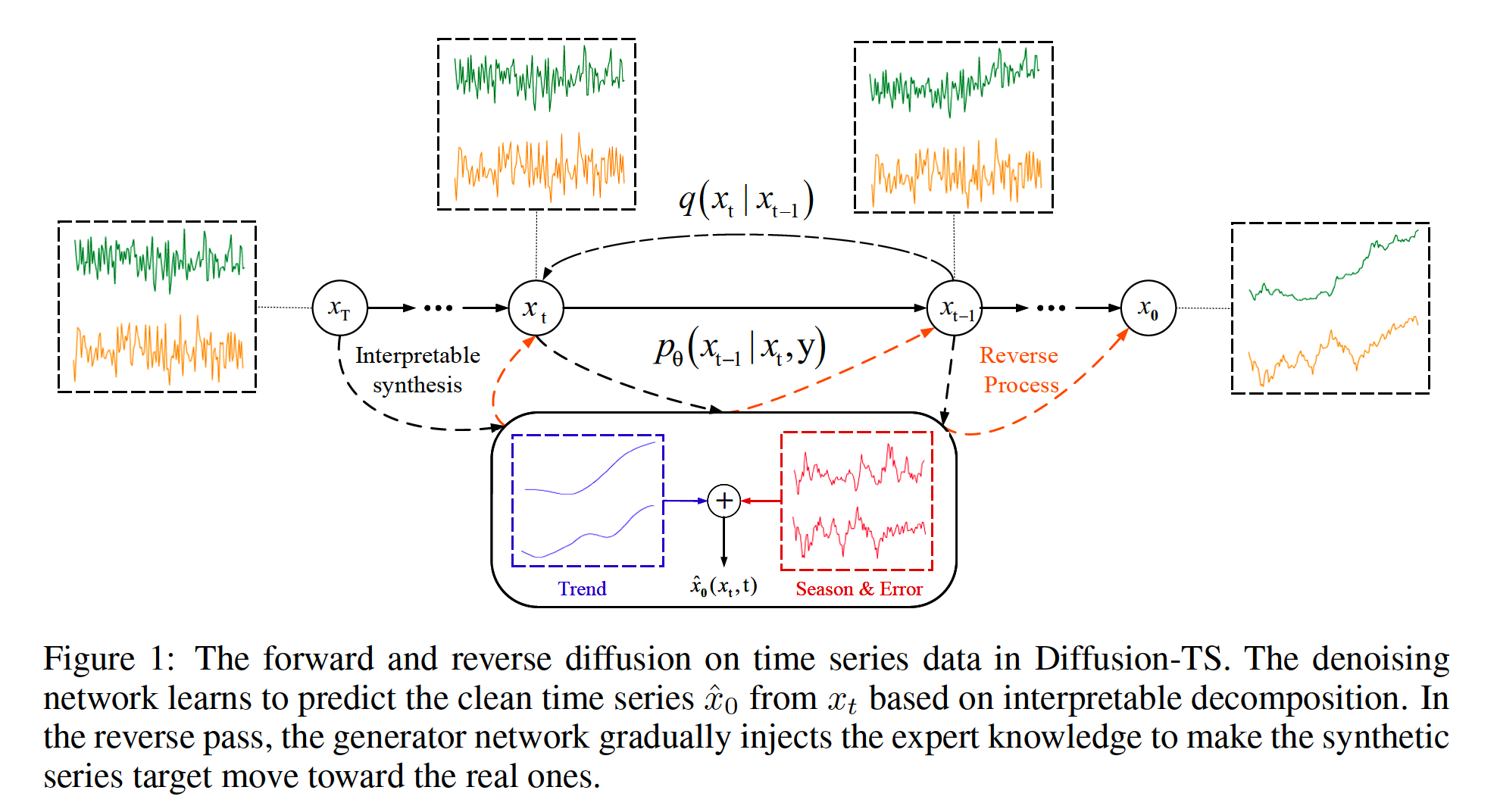
(1) Diffusion Framework

Predict the “data” instead of noise

• \(\mathcal{L}\left(x_0\right)=\sum_{t=1}^T \underset{q\left(x_t \mid x_0\right)}{\mathbb{E}} \mid \mid \mu\left(x_t, x_0\right)-\mu_\theta\left(x_t, t\right) \mid \mid ^2\).

(2) Model Structure

Transformer …. renovate decoder: use interpretable layers

• (1) Trend synthetic layer
• (2) Fourier synthetic layer

a) Trend Synthesis

Trend = slow-varying behavior

Polynomial regressor

• \(V_{t r}^t=\sum_{i=1}^K\left(\mathbf{C} \cdot \operatorname{Linear}\left(w_{t r}^{i, t}\right)+\mathcal{X}_{t r}^{i, t}\right), \quad \mathbf{C}=\left[1, c, \ldots, c^p\right]\).

  • \(w_{(\cdot)}^{i, t}\): Input of interpretable layers

    • where $i \in 1, \ldots, K$ denotes the index of the corresponding decoder block at diffusion step $t$.

  • \(\mathcal{X}_{t r}^{i, t}\) : Mean value of the output of the \(i^{t h}\) decoder block

  • \(\mathbf{C}\) : Slow-varying poly space

    ( = matrix of powers of vector \(c=[0,1,2, \ldots, \tau-2, \tau-1]^T / \tau\) )

  • \(p\) : Small degree (e.g. \(p=3\) ) to model low frequency behavior.

b) Seasonality & Error Synthesis

Recover other components other than trends

Inspired by the trigonometric representation of seasonal components based on Fourier series

\(\rightarrow\) Use Fourier bases

\(\begin{gathered} A_{i, t}^{(k)}= \mid \mathcal{F}\left(w_{\text {seas }}^{i, t}\right)_k \mid , \Phi_{i, t}^{(k)}=\phi\left(\mathcal{F}\left(w_{\text {seas }}^{i, t}\right)_k\right), \\ \kappa_{i, t}^{(1)}, \cdots, \kappa_{i, t}^{(K)}=\underset{k \in\{1, \cdots,\lfloor\tau / 2\rfloor+1\}}{\arg \operatorname{TopK}}\left\{A_{i, t}^{(k)}\right\}, \\ S_{i, t}=\sum_{k=1}^K A_{i, t}^{\kappa_{i, t}^{(k)}}\left[\cos \left(2 \pi f_{\kappa_{i, t}^{(k)}} \tau c+\Phi_{i, t}^{\kappa_{i, t}^{(k)}}\right)+\cos \left(2 \pi \bar{f}_{\kappa_{i, t}^{(k)}} \tau c+\bar{\Phi}_{i, t}^{\kappa_{i, t}^{(k)}}\right)\right], \end{gathered}\).

c) Final Result

\(\hat{x}_0\left(x_t, t, \theta\right)=V_{t r}^t+\sum_{k=1}^K S_{i, t}+R\).

• \(R\): output of the last decoder block

  ( = sum of residual periodicity and other noise )

(3) Fourier-based Training Objective

Guide the interpretable diffusion training by applying it into frequency domain (with FFT)

\(\mathcal{L}_\theta=\mathbb{E}_{t, x_0}\left[w_t\left[\lambda_1 \mid \mid x_0-\hat{x}_0\left(x_t, t, \theta\right) \mid \mid ^2+\lambda_2 \mid \mid \mathcal{F} \mathcal{F} \mathcal{T}\left(x_0\right)-\mathcal{F} \mathcal{F} \mathcal{T}\left(\hat{x}_0\left(x_t, t, \theta\right)\right) \mid \mid ^2\right]\right]\).

(4) Conditional Generation for TS Applications

(Above: UNconditional TS generation)

Conditional TS generation

• i.e. forecasting, imputation

• modeled \(x_0\) is conditioned on targets \(y\).

Dhariwal & Nichol (2021)

• Gradient-guided way to overcome this limitation
• Pre-trained diffusion model can be conditioned using the gradients of a classifier

\(\tilde{x}_0\left(x_t, t, \theta\right)=\hat{x}_0\left(x_t, t, \theta\right)+\eta \nabla_{x_t}\left( \mid \mid x_a-\hat{x}_a\left(x_t, t, \theta\right) \mid \mid _2^2+\gamma \log p\left(x_{t-1} \mid x_t\right)\right)\).

• conditional part \(x_a\) & generative part \(x_b\)
• gradient term = reconstruction-based guidance, with \(\eta\) controlling the strength