T-Rep: Representation Learrning for TS using Time-Embeddings
Contents
- Abstract
- Introduction
- Background
- Method
- Encoder
- Pretext Tasks
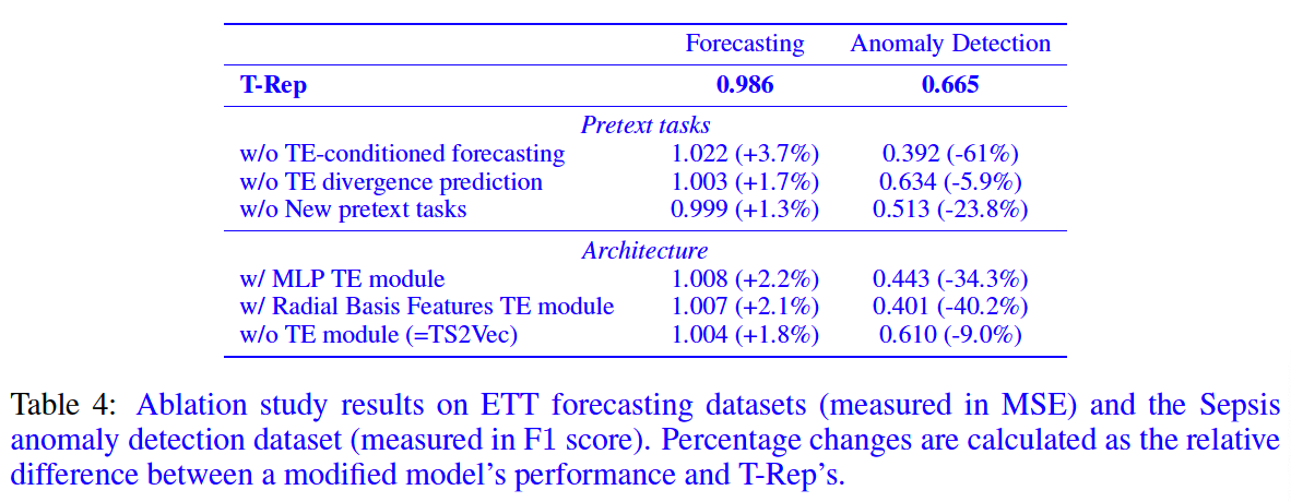
- Experiments
Abstract
MTS = unlabeld, high-dim, noisy, missing data ..
\(\rightarrow\) Solution: T-Rep
- SSL method to learn TS representations at a timestep granuality
- Learn vector embeddings of TIME
-
Pretext tasks: to incorporate smooth & fine-grained temporal dependencies
- Experiments: cls, fcst, ad
1. Introduction
TS2Vec: instance-level & tilmestep-level
Central issue in RL in TS: incorporation of time in the latent space
T-Rep
-
Improves the treatment of time in SSL thanks to the use of time-embeddings
- integrated in the feature-extracting encoder & leveraged in the pretext teasks
-
Time-embedding
- a vector embedding of time
- obtained as the output of a learned function \(h_\psi\),
- encodes temporal signal features such as trend, periodicity, distribution shifts
\(\rightarrow\) enhance our model’s resilience to missing data & non-stationarity
2. Background
(1) Problem Definitions
- \(X=\left\{\mathbf{x}_1, \ldots, \mathbf{x}_N\right\} \in \mathbb{R}^{N \times T \times C}\) .
- Embedding function \(f_\theta\), s.t. \(\forall i \in[0, N]\)
- \(\mathbf{z}_i=f_\theta\left(\mathbf{x}_i\right)\), where \(\mathbf{z}_i \in \mathbb{R}^{T \times F}\)
(2) Contextual Consistency
- Instance-wise CL
- Temporal CL
(3) Hierarchical CL
pass
3. Method
(1) Encoder
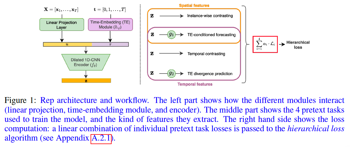
a) Linear Projection Layer
-
\(\mathbf{x}_{i, t} \in \mathbb{R}^C\) to vectors \(\mathbf{u}_{i, t} \in \mathbb{R}^F\)
-
After linear projection) Random timestamp masking to each \(\mathbf{u}_i\) ( like TS2Vec )
s
b) Time-Embedding Module \(h_\psi\)
-
Responsible for learning time-related features \(\tau_t\) (trend, periodicity, distribution shifts etc.) directly from the TS sample indices \(t\).
-
Not fixed like a transformer’s positional encoding module
( Instead, learned jointly with the rest of the encoder )
-
Recommend using Time2Vec
- captures trend and periodicity
\(\rightarrow\) T-Rep = first model to combine a time-embedding module & CNN in SSL
Output of time-embedding module
-
Probability distribution ( sum = 1 )
- reason) use of statistical divergence measures in a pretext task
-
\(\left(\boldsymbol{\tau}_t\right)_k=\frac{\sigma\left(h_\psi(t)\right)_k}{\sum_{j=1}^K \sigma\left(h_\psi(t)\right)_j}\).
- where \(\boldsymbol{\tau}_t\) contains \(K\) elements
-
Time-embeddings \(\boldsymbol{\tau}_t\) are concatenated with vectors \(\mathbf{u}_{i, t}\) after the linear projection
\(\rightarrow\) Vectors \(\left[\mathbf{u}_{i, t} \boldsymbol{\tau}_t\right]^T\) are fed to the encoder \(f_\theta\).
c) TCN Encoder
Pass
(2) Pretext Tasks
- (1) Time-Embedding Divergence Prediction
- how the information gained through time-embeddings should structure the latent space and be included in the time series representations.
- (2) Time-embedding-conditioned Forecasting
- what information the time-embeddings and representations should contain.
a) Time-Embedding Divergence Prediction
-
Goal: integrate the notion of time in the latent space
-
Key : divergence measure between two time-embeddings \(\tau\) and \(\boldsymbol{\tau}^{\prime}\)
-
Purpose: distances in the latent space to correlate with temporal distances
\(\rightarrow\) smoother latent trajectories than with CL
Notation:
-
Regression Task
- Batch \(X \in \mathbb{R}^{B \times T \times C}\),
- sample \(\mathbf{x}_{i, t}\) and \(\mathbf{x}_{j, t^{\prime}} \forall i, j \in[0, B]\) and \(t, t^{\prime} \in[0, T]\) s.t. \(t \neq t^{\prime}\).
- Task input : \(\mathbf{z}_{i, t}-\mathbf{z}_{j, t^{\prime}}^{\prime}\),
- Regression target : \(y=\mathcal{D}\left(\tau, \boldsymbol{\tau}^{\prime}\right)\)
- \(\boldsymbol{\tau}\) and \(\boldsymbol{\tau}^{\prime}\) are the respective time-embeddings of \(t\) and \(t^{\prime}\),
- \(\mathcal{D}\) : measure of statistical divergence … use JSD
Loss : \(\mathcal{L}_{\text {div }}=\frac{1}{M} \sum_{\left(i, j, t, t^{\prime}\right) \in \Omega}^M\left(\mathcal{G}_1\left(\mathbf{z}_{i, t}-\boldsymbol{z}_{j, t^{\prime}}^{\prime}\right)-J S D\left(\boldsymbol{\tau}_t \mid \mid \boldsymbol{\tau}_{t^{\prime}}\right)\right)^2\).
- where \(\Omega\) is the set (of size \(M\) ) of time/instance indices for the randomly sampled pairs of representations
Using divergences ( instead of simple norm
- ex) suppose the time-embedding is a 3-dimensional vector that learned a hierarchical representation of time (equivalent to seconds, minutes, hours). A difference of 1.0 on all time scales \((01: 01: 01\) ) represents a very different situation to a difference of 3.0 hours and no difference in minutes and seconds (03:00:00), but could not be captured by a simple vector norm.
b) Time-Embedding Conditioned Forecasting
Goal: incorporate predictive information & encourage robustness to missing data
Key:
- Input) representation of TS at specific timestep
- Output) predict the representation vector of nearby point
Notation
- Input: concatenation \(\left[\mathbf{z}_{i, t} \boldsymbol{\tau}_{t+\Delta}\right]^T\) of
- the representation \(\mathbf{z}_{i, t} \in \mathbb{R}^F\) at time \(t\)
- the time-embedding of the target \(\tau_{t+\Delta} \in \mathbb{R}^K\)
- \(\Delta_{\max }\) : hyperparameter to fix the range in which the prediction target can be sampled
- Target: \(\mathbf{z}_{i, t+\Delta}\)
- at a uniformly sampled timestep \(t+\Delta, \Delta \sim \mathcal{U}\left[-\Delta_{\max }, \Delta_{\max }\right]\).
- Task head: \(\mathcal{G}_2: \mathbb{R}^{F+K} \mapsto \mathbb{R}^F\), a 2-layer MLP with ReLU
Loss (MSE):
- \(\mathcal{L}_{\text {pred }}=\frac{1}{M T} \sum_{j \in \Omega_N}^M \sum_{t \in \Omega_T}^T\left(\mathcal{G}_2\left(\left[\begin{array}{ll}
\mathbf{z}_{i, t}^{\left(c_1\right)} & \boldsymbol{\tau}_{t+\Delta_j}
\end{array}\right]^T\right)-\mathbf{z}_{i, t+\Delta_j}^{\left(c_2\right)}\right)^2\).
- where \(\Delta_j \sim \mathcal{U}\left[-\Delta_{\max }, \Delta_{\max }\right], \Omega_M\) and \(\Omega_T\) are the sets of randomly sampled instances and timesteps for each batch
4. Experiments