METRO : A Generic GNN Framework for MTS Forecasting (2020, 131)Permalink

ContentsPermalink

1. Abstract
2. Introduction
3. Preliminaries
4. METRO
   1. Temporal Graph Embedding Unit
   2. Single-scale Graph Update Unit
   3. Cross-scale Graph Fusion Kernel
   4. Predictor and Training Strategy

0. AbstractPermalink

METROPermalink

• generic framework with “Multi-scale Temporal Graphs NN”

• models the “dynamic & cross-scale variable correlations” simultaneously

• represent MTS as “series of temporal graphs”

  can capture both

  • inter-step correlation
  • intra-step correlation

  via message-passing & node embedding

1. IntroductionPermalink

GNN for MTS forecasting

• capture the interdependencies & dynamic trends over a group of variables

  • nodes = variables
  • edges = interactions of variables

• can use “even for data w.o explicit graph structures”

  • use hidden graph structures

• previous works

  • assume that “MTS are static”

    $\rightarrow$ however, “interdependencies between variables can be temporally dynamic”

    • ex) MTGNN, TEGNN, ASTGCN

Previous GNN works

• MTGNN & TEGNN

  • learn/compute adjacency matrices of graphs, from the whole input TS
  • hold them for “subsequent temporal modeling”

• ASTGCN

  • for ‘traffic prediction’

    ( connections between nodes are known in advance )

  • considers “adaptive adjacency matrix” ( attention value )

  • but on relatively large scale, that only cahnges with regard to input series example

• STDN

  • flow gating mechanism, to learn “dynamic similarity” by time step
  • but, can only be applied on consecutive & grid partitioned regional maps

Multi-scale patterns

• [ approach 1 ]

  • treat time stamps of MTS as “side information”
  • combine the “embedded time stamps” with MTS’s embedding

• [ approach 2 ]

  • first, adopt filters ( with different kernel sizes ) to MTS
  • second, sum/concatenate the multi-scale features

• common

  • can incorporate information “across different scales”

  • but, just simple linear-weight transformation

    ( relation between pairs of scales are ignored )

Problems

• 1) dependencies between variables are dynamic
• 2) temporal patterns in MTS occur in multiple scale

$\rightarrow$ propose METRO ( Multi-scalE Temporal gRaph neurla netwOrks )

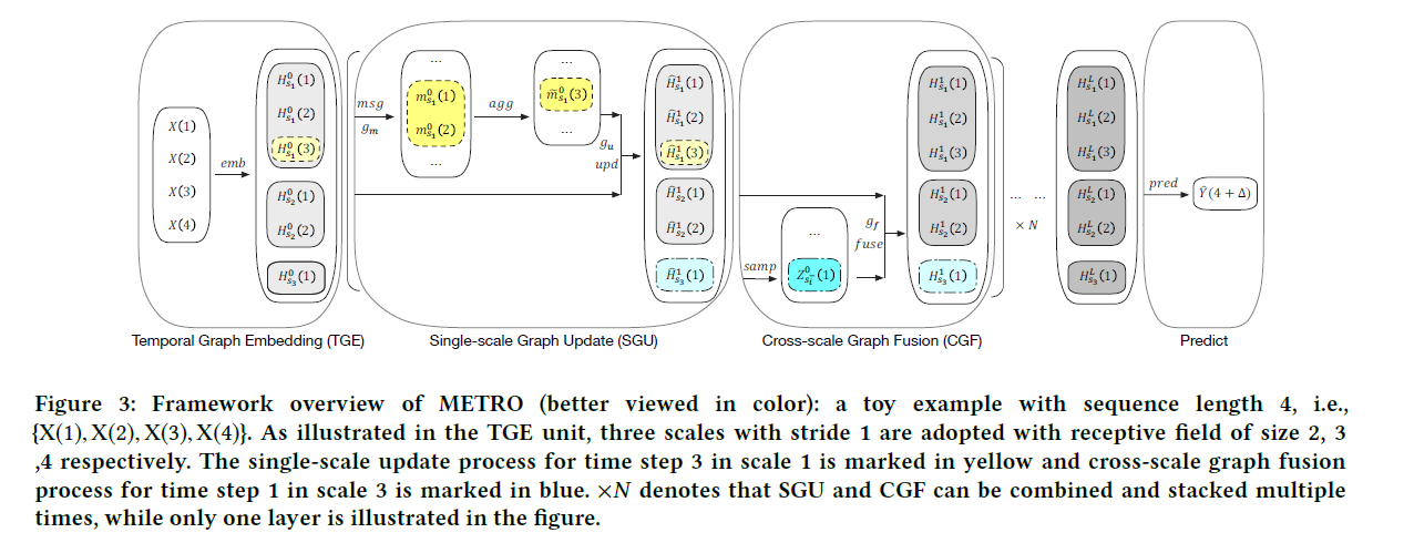
4 components of METRO

• 1) TGE (Temporal Graph Embedding)
  • obtains “node embeddings” under multi-scale
• 2) SGU (Single-scale Graph Update)
  • dynamically leverages graph structures of nodes in each single scale
  • propagates info from a node’s intra/inter-step neighbors
• 3) CGF (Cross-scale Graph Fusion) kernel
  • walks along the time axis & fuses features across scales
• 4) predictor
  • decoder ( decodes node embeddings )
  • gives final predictions

2. PreliminariesPermalink

MTS forecastingPermalink

Notation

• MTS : $X=\{X(1), X(2), \ldots, X(t)\}$
  • at time $i$ : $X(i)=\left[x_{i, 1}, . ., x_{i, n}\right] \in \mathbb{R}^{n \times m}, i \in[1, \ldots, t]$.
    • $x_{i, k} \in \mathbb{R}^{m}, k \in[1, \ldots, n]$.
  • $n$ : number of variables ( TS )
  • $m$ : number of dimension
• Goal : predict $\Delta$ steps ahead
  • output : $\hat{Y}(t+\Delta)=X(t+\Delta)=\left[x_{t+\Delta, 1}, . ., x_{t+\Delta, n}\right]$
  • input : $\{X(t-w+1), \ldots, X(t)\}$

GraphsPermalink

(1) Graph : $G=(V, E)$

• static graph
• vertices & edges are invariant over time

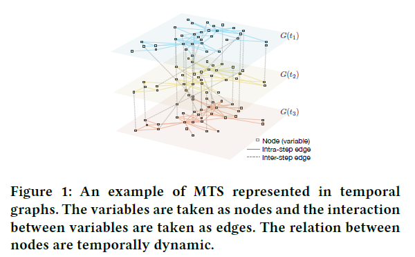
(2) Temporal Graph : $G(t)=(V(t), E(t))$

• graph as a function of time
• 2 types of temporal graphs
  • 1) INTRA-step TG : $V(t)$ is made up of variables within time step $t$
  • 2) INTER-step TG : $V(t)$ consists variables of time step $t$ and its previous time step $t-1$

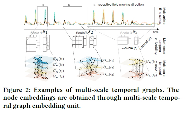
(3) Multi-scale Temporal Graph : $G_{S}(t)=\left(V_{S}(t), E_{S}(t)\right)$

• each node in the graph represents an observation of “time-length $w_s$”

3. METROPermalink

(1) TGE (Temporal Graph Embedding Unit)Permalink

TGE = “encoder”

• obtain “embeddings of TEMPORAL features of each variables”

• example)

  • input : $\left\{X\left(t_{0}\right), \ldots\right.\left.X\left(t_{0}+w-1\right)\right\}$

  • output :

    • temporal feature at time step $\mathrm{t}, t \in\left[t_{0}, \ldots, t_{0}+\right.$ $w-1]$,

      under scale $i$ is..

    • $\mathrm{H}_{s_{i}}^{0}(t)=\operatorname{emb}\left(s_{i}, t\right)=f\left(X(t), \ldots, X\left(t+w_{s_{i}}-1\right)\right)$.

  • notation

    • $n$ : # of variables

    • $d$ : embedding dimension

    • $f$ : embedding function

      • ex) unpadded convolution with multiple filters with size $1 \times w_{s_i}$

        ( output of multiple convolution channels are “concatenated” )

(2) SGU (Single-scale Graph Update Unit)Permalink

modeling “hidden relations among variables”

• by training/updating “adjacency matrices”
• problem : message aggregation over time, with FIXED structures?

Solution : introduce SGU

• adaptively learn “INTRA & INTER” step adjacency matrix of variables

• propose “graph-based temporal message passing”

  • use “historical temporal information” of nodes

• ex) SGU operates $s_1$, $s_2$, $s_3$ separately

  

• example : $G_{s_1}(:)$ … jointly considers

  • 1) message passing WITHIN a time step
    • $G_{s_1}(t_i)$ & time stamps
  • 2) message passing BETWEEN a time step
    • $G_{s_1}(t_i)$ & $G_{s_1}(t_2)$

Process

• 1) learn messages

  • messages between nodes of 2 adjacent time steps :

    • $\mathbf{m}^{l}(t-j)=m s g\left(\mathbf{H}^{l}(t-j-1), \mathbf{H}^{l}(t-j), A_{t-j-1, t-j}^{l}\right)$.

      where $A_{t-j-1, t-j}^{l}=g_{m}\left(\mathbf{H}^{l}(t-j-1), \mathbf{H}^{l}(t-j)\right)$.

  • ex) $msg$ : GCN

  • ex) $g_m$ : transfer entropy / node-embedding-based deep layer model

• 2) aggregate messages

  • $\widetilde{\mathbf{m}}^{l}(t)=\operatorname{agg}\left(\mathbf{m}^{l}(t-k-1), \ldots, \mathbf{m}^{l}(t-1)\right)$.
  • ex) simple concatenation / RNN / Transformer …

Update

• embedding of nodes ( in step $t$ ) are updated, based on..

  • 1) aggregated message
  • 2) memory of previous layer

• $\hat{\mathrm{H}}^{l+1}(t) =u p d\left(\widetilde{\mathrm{m}}^{l}(t), \mathbf{H}^{l}(t), A_{t}^{l}\right)$.

  where $A_{t}^{l} =g_{u}\left(\widetilde{\mathrm{m}}^{l}(t), \mathbf{H}^{l}(t)\right)$

  • ex) $upd$ : memory update function ( GRUs, LSTMs )
  • ex) $g_u$ : graph-based GRU

(3) CGF (Cross-scale Graph Fusion) KernelPermalink

CGF

• diffuse information “ACROSS SCALES”
• “scales” = ‘size of respective fields’
• need to decide “which time steps in which scales” can interact

Standard = “HIGHER scale”

Sampling fine features (time steps) = “LOWER scales”

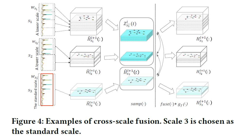
• $\mathrm{Z}_{s_{i}^{-}}^{l}(t)=\operatorname{samp}\left(\hat{\mathbf{H}}_{s_{1}}^{l+1}(:), \ldots, \hat{\mathbf{H}}_{s_{i-1}}^{l+1}(:)\right)$.
  • $\hat{\mathbf{H}}_{s_{j}}^{l+1}(:)$ : output updated features of SGU unit
  • $\mathrm{Z}_{s_{i}^{-}}^{l}$ : selected lower scale features, concatenated in time axis

Information diffusion, between

• 1) $\mathrm{Z}_{s_{i}^{-}}^{l}(t)$
• 2) $\hat{\mathbf{H}}_{s_{i}}^{l+1}(t)$

using a graph learning function $g_f$

$\begin{aligned} \mathrm{H}_{s_{1}: s_{i-1}}^{l+1}(:), \mathrm{H}_{s_{i}}^{l+1}(t) & \leftarrow f u s e\left(\mathrm{Z}_{s^{-}}^{l}(t), \hat{\mathrm{H}}_{s_{i}}^{l+1}(t), A_{\left(s_{i}^{-}, s_{i}\right), t}^{l}\right), \\ A_{\left(s_{i}^{-}, s_{i}\right), t}^{l} &=g_{f}\left(\mathrm{Z}_{s_{i}^{-}}^{l}(t), \hat{\mathrm{H}}_{s_{i}}^{l+1}(t)\right), \end{aligned}$.

• $\mathrm{H}_{s_{1}: s_{i-1}}^{l+1}(:)$ : cross-scale fused embedding of sampled lower scale features
• $\mathbf{H}_{s_{i}}^{l+1}(t)$ : standard high scale at time step $t$
• ex) $fuse$ : GCNs

(4) Predictor and Training StrategyPermalink

$\hat{Y}(t+\Delta)=\operatorname{pre}\left(\mathbf{H}_{s_{1}: s_{p}}(:)\right)$.