(paper) Discrete Graph Structure Learning for Forecasting Multiple Time Series

Discrete Graph Structure Learning for Forecasting Multiple Time Series (2021, 11)

Contents

1. Abstract
2. Introduction
3. Related Work
4. Method
   1. Graph Structure Parameterization
   2. GNN Forecasting
   3. Training, optionally with a Priori Knowledge of the graph

0. Abstract

pairwise information among MTS

\(\rightarrow\) use GNN to capture!

Propose

• learning the “STRUCTURE” simultaneously with “GNN”

• cast the problem as..

  • learning a probabilistic graph model,

    through optimizing the mean performance over the graph distribution

1. Introduction

MTS forecasting

• “interdependency” among variables are imporatnt!
• GNN approaches
  • 1) GCRN
    • Structured sequence modeling with graph convolutional recurrent networks
  • 2) DCRNN
    • Diffusion convolutional recurrent neural network: Data-driven traffic forecasting
  • 3) STGCN
    • Spatio-temporal graph convolutional networks: A deep learning framework for traffic forecasting
  • 4) T-GCN
    • T-GCN: A temporal graph convolutional network for traffic prediction

But, graphs structures are not always available!

\(\rightarrow\) LDS ( solve ase bilevel program )

Problems of LDS

• 1) computationally expensive ( inner & outer objective )
• 2) challenging to scale

\(\rightarrow\) this paper uses “UNI-level optimization”

proposes GTS (Graph for Time Series)

• (LDS) inner optimization \(w(\theta)\)
• (GTS) paramterization \(w(\theta)\)

2. Related Work

GNN for time series

• GCRN, DCRNN, STGCN, T-GCN
  • combine “temporal recurrent processing” with GCN to augment representation learning of individual TS

• MTGNN

  • parameterizes the graph as a degree-\(k\) graph,

    learned end-to-end with a GNN for TS forecasting

• NRI

  • adopts a latent-variable approach
  • learns a latent graph for forecasting system dynamics

3. Method

Notation

• \(X\) : training data
  • 3 dimensional tensor
    • 1) feature
    • 2) time
    • 3) \(n\) series
      • \(X^i\) : \(i\)-th series
• \(S\) : total time steps
  • \(T\) : window size
  • \(\tau\) : forecasting horizon
• \(\widehat{X}_{t+T+1: t+T+\tau}=f\left(A, w, X_{t+1: t+T}\right)\).
• training objective :
  • \(\sum_{t} \ell\left(f\left(A, w, X_{t+1: t+T}\right), X_{t+T+1: t+T+\tau}\right)\).

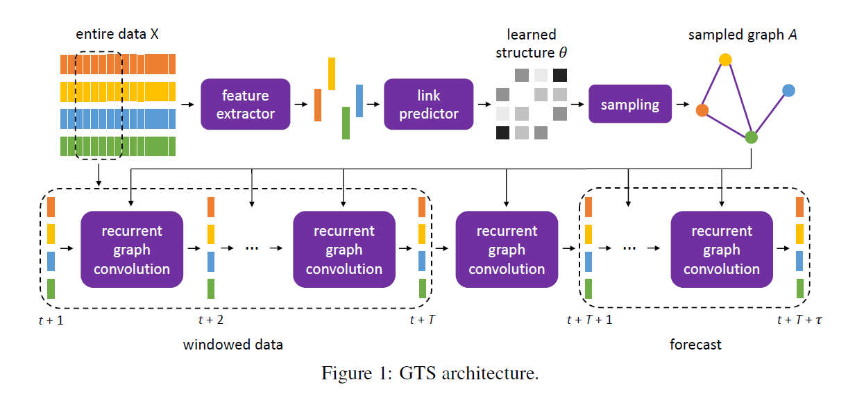
(1) Graph Structure Parameterization

Binary matrix \(A \in\{0,1\}^{n \times n}\)

\(\rightarrow\) let \(A\) be a r.v of matrix Bernoulli distn

• parameterized by \(\theta \in[0,1]^{n \times n}\)
• \(A_{i j}\) is independent for all the \((i, j)\) pairs with \(A_{i j} \sim \operatorname{Ber}\left(\theta_{i j}\right) .\)

Training Objective

• (before) \(\sum_{t} \ell\left(f\left(A, w, X_{t+1: t+T}\right), X_{t+T+1: t+T+\tau}\right)\)
• (after) \(\mathrm{E}_{A \sim \operatorname{Ber}(\theta)}\left[\sum_{t} \ell\left(f\left(A, w, X_{t+1: t+T}\right), X_{t+T+1: t+T+\tau}\right)\right]\).

Gumbel reparameterization trick

• \(A_{i j}=\operatorname{sigmoid}\left(\left(\log \left(\theta_{i j} /\left(1-\theta_{i j}\right)\right)+\left(g_{i j}^{1}-g_{i j}^{2}\right)\right) / s\right)\),

  where \(g_{i j}^{1}, g_{i j}^{2} \sim \operatorname{Gumbel}(0,1)\) for all \(i\), \(j\)

For parameterization of \(\theta\)…use

• 1) feature extractor ( \(X^{i}\) \(\rightarrow\) \(z^{i}\) )
  • make feature vector for each TS
  • \(z^{i}=\operatorname{FC}\left(\operatorname{vec}\left(\operatorname{Conv}\left(X^{i}\right)\right)\right)\).
• 2) link predictor ( \(\left(z^{i}, z^{j}\right) \rightarrow \text{scalar} \theta_{i j} \in[0,1]\) )
  • input : pair of feature vectors
  • output : link probability
  • \(\theta_{i j}=\operatorname{FC}\left(\operatorname{FC}\left(z^{i} \mid \mid z^{j}\right)\right)\).

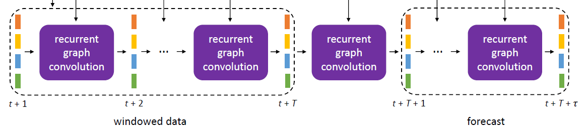
(2) GNN Forecasting

• use “seq2seq”

  • for each TS \(i\) … map \(X_{t+1: t+T}^{i}\) to \(X_{t+T+1: t+T+\tau}^{i}\)
  • with “GCN” version

• Encoder

  • Encoder Input : \(X_{t^{\prime}}\) for all series
  • Process : updates the internal hidden state from \(H_{t^{\prime}-1}\) to \(H_{t^{\prime}}\)
  • Encoder output : \(H_{t+T}\) ( = summary of input )

• Decoder

  • Decoder Input : \(H_{t+T}\)
  • Process : evolves the hidden state for another \(\tau\) steps
  • Decoder Outputs :
    • Each hidden state \(H_{t^{\prime}}, t^{\prime}=t+T+1: t+T+\tau\), simultaneously serves as the output \(\widehat{X}_{t^{\prime}}\)
    • becomes input to the next time step

• use “diffusion convolutional GRU” in DCRNN

  ( = designed for “directed graphs” )

(3) Training, optionally with a Priori Knowledge of the graph

(a) Base Training Loss

• per window
• use MAE
• \(\ell_{\text {base }}^{t}\left(\widehat{X}_{t+T+1: t+T+\tau}, X_{t+T+1: t+T+\tau}\right)=\frac{1}{\tau} \sum_{t^{\prime}=t+T+1}^{t+T+\tau} \mid \widehat{X}_{t^{\prime}}-X_{t^{\prime}} \mid\).

(b) Regularization

• sometimes, actual graph among TS is known ( ex. Traffic Network )

• also, “neighborhood graph” ( ex. kNN ) may still serve as a reasonable knowledge

  \(\rightarrow\) can be prior graph \(A^a\)

• use CE loss, between \(\theta\) & \(A^a\)

• \(\ell_{\text {reg }}=\sum_{i j}-A_{i j}^{\mathrm{a}} \log \theta_{i j}-\left(1-A_{i j}^{\mathrm{a}}\right) \log \left(1-\theta_{i j}\right) \text {. }\).

Overall Training Loss = \(\sum_{t} \ell_{\text {base }}^{t}+\lambda \ell_{\text {reg }}\).