(paper) Spectral Temporal GNN for MTS Forecasting

Spectral Temporal GNN for MTS Forecasting (2021, 41)

Contents

1. Abstract
2. Introduction
3. Related Work
4. Problem Definition
5. StemGNN ( Spectral Temporal GNN )
   1. Overview
   2. Latent Correlation Layer
   3. StemGNN Block

0. Abstract

Captures both

• 1) temporal correlations ( in time domain )
• 2) inter-series correlation

jointly, in the “spectral domain”

Combines

• 1) GFT (Graph Fourier Transform) \(\rightarrow\) inter-series correlation
• 2) DFT (Discrete Fourier Transform) \(\rightarrow\) temporal correlations

in an end-to-end framework

1. Introduction

previous works

• SFM (State Frequency Memory) network :
  • combines DFT & LSTM for stock price prediction
• SR (Spectral Residual) model :
  • leverages DFT in anomaly detection
• traffic forecasting
  • model correlations among “multiple TS”
  • ex) GCNs based models : stack GCN & temporal modules (LSTM,GRU)
    • only caputre “temporal pattenrs” in time domain
    • also, require pre-defined topology of inter-series relationshisp

This paper models

• 1) intra-series temporal patterns
• 2) inter-series temporal patterns

StepGNN

• combines both DFT & GFT

• model MTS data in “spectral domain”
  • spectral representations : clearer patterns & predicted more efficiently
• StemGNN block
  • step 1) GFT : transfer structural MTS into “spectral TS”
    • different trends can be decomposed to orthogonal TS
  • step 2) DFT : transfer each univariate TS into “frequency domain”
  • then, spectral representation becomes easier to be recognized by convolution & sequential modeling layers
• adopt both “forecasting & backcasting” output modules, with shared encoders

2. Related Work

MTS

• TCN
  • treats high-dim data entirely as a tensor input
  • considers a “large receptive field” through dilated CNN
• LSTNet
  • CNN + RNN to extract…
    • 1) short-term local dependence patterns among variables
    • 2) long-term patterns of TS
• DeepState
  • state-space models with deep RNN
• DeepGLO
  • leverages both global & local features during training/forecasting
  • based on “matrix factorization”

MTS + GNN

• DCRNN

  • for traffic forecasting
  • incorporate both “spatial & temporal” dependencies in convolutional RNN

• ST-GCN

  • for traffic forecasting

  • integrates “graph convolution” & “gated temporal convolution”,

    through “spatio-temporal convolutional blocks”

• Graph WaveNet

  • combines graph convolutional layers with..

    • “adaptive adjacency matrices”
    • dilated causal convolutions

    to capture “spatio-temporal dependencies”

\(\rightarrow\) but all those ignore “INTER-series correlation” ( or require dependency graph as priors )

& not in spectral domain

3. Problem Definition

Multivariate Temporal Graph : \(\mathcal{G}=(X, W)\)

• MTS input : \(X=\left\{x_{i t}\right\} \in \mathbb{R}^{N \times T}\).
  • \(N\) : # of time series (nodes)
  • \(T\) : # of time stamps
  • \[X_{t} \in \mathbb{R}^{N}\]
• Adjacency matrix : \(W \in \mathbb{R}^{N \times N}\)

Task :

• input : previous \(K\) time stamps
  • \(X_{t-K}, \cdots, X_{t-1}\).
• output : next \(H\) time stamps
  • \(\hat{X}_{t}, \hat{X}_{t+1}, \cdots, \hat{X}_{t+H-1}\).
• model :
  • \(\hat{X}_{t}, \hat{X}_{t+1} \ldots, \hat{X}_{t+H-1}=F\left(X_{t-K}, \ldots, X_{t-1} ; \mathcal{G} ; \Phi\right)\).
    • \(F\) : forecasting model, with parameter \(\Phi\)
    • \(\mathcal{G}\) : graph structure ( can be input as prior, or automatically inferred )

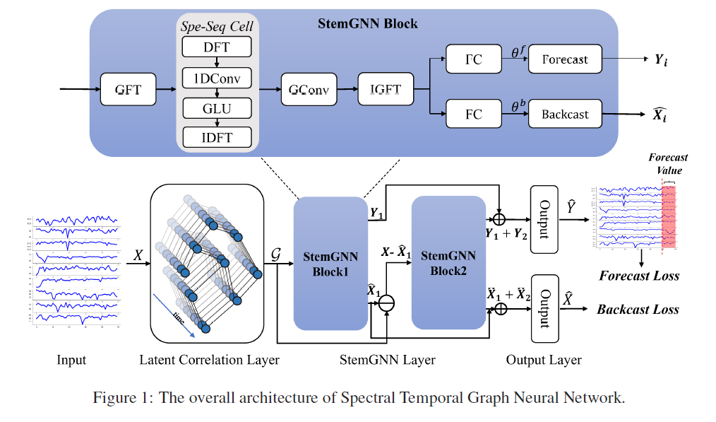
4. StemGNN ( Spectral Temporal GNN )

(1) Overview

StemGNN

• a general solution for MTS
• 3 steps
  • 1) latent correlation layer
    • input : \(X\)
    • output : graph structure & weight matrix \(W\) is inferred
  • 2) StemGNN Layer
    • input : graph \(\mathcal{G}=(X,W)\)
    • layer : consists of 2 residual StemGNN blocks
      • designed to model “structural & temporal” dependencies inside MTS, in spectral domain
        • 1) GFT
        • 2) DFT
        • 3) 1D conv & GLU sub layers
        • 4) inverse DFT
        • 5) graph convolution
        • 6) inverse GFT
  • 3) output layer
    • composed of GLU & FC
    • 2 kinds of output
      • 1) forecasting outputs \(Y_i\)
      • 2) backcasting outputs \(\hat{X_i}\)
• Loss Function
  • \(\mathcal{L}\left(\hat{X}, X ; \Delta_{\theta}\right)=\sum_{t=0}^{T} \mid \mid \hat{X}_{t}-X_{t} \mid \mid _{2}^{2}+\sum_{t=K}^{T} \sum_{i=1}^{K} \mid \mid B_{t-i}(X)-X_{t-i} \mid \mid _{2}^{2}\).
• Inference : “rolling strategy for multi-step prediction”

(2) Latent Correlation Layer

Input : \(X \in \mathbb{R}^{N \times T}\)

Layer : GRU

• use the last hidden state \(R\) as the representation of entire TS
• calculate weight matrix \(W\) by self attention
  • \(Q=R W^{Q}, K=R W^{K}, W=\operatorname{Softmax}\left(\frac{Q K^{T}}{\sqrt{d}}\right)\).
• \(W \in \mathbb{R}^{N \times N}\) : served as “adjacency matrix”

(3) StemGNN Block

( StemGNN layer = multiple StemGNN blocks + skip connections )

StemGNN Block

• designed by embedding a Spe-Seq (Spectral Sequential) Cell,
• into a Spectral Graph Convolution module

Described in picture above!

• Spectral Graph Convolution : learn latent representation of MTS in spectral domain

• GFT : capture inter-series relationships

  • output of GFT is also MTS

• DFT : capture repeated patterns in periodic data

  ( auto-correlation features among different time stamps )