(paper) Deep Gate ; Global-local decomposition for MTS modeling

Deep Gate : Global-local decomposition for MTS modeling (2022)

Contents

1. Abstract
2. Introduction
3. Motivation
4. Proposed Method
   1. Problem Formulation
   2. Global-local decomposition
   3. Deep Gate
      1. Decomposition module
      2. Prediction module
   4. Denoting training technique
   5. Training method

0. Abstract

MTS = have common dynamics

( stem from “global factors ” )

Shared information from “global components” \(\rightarrow\) enhance forecasting performance

BUT…existing methods…

• treat global factors as additiona hidden states INSIDE the model

Deep Gate

• “explicit” global-local decomposition
• employ a “denoising” training technique for multi-step forecasting problems

1. Introduction

Contributions.

• (1) simple / effective global-local framework for MTS modeling

  • models global & local “separately”

• (2) first decomposes the underlying global & local series

  & transers them to predict future global & local values

2. Motivation

STL decomposition

• most popular decomposition moethods
• BUT…limited to “univariate” TS & do not facilitate the dependencies between individual TSs

MTS have “common behaviors”

• BUT…previous works treat common behavior as “intermediate hidden features”, IMPLICITLY

  \(\rightarrow\) can not be utilized as “decomposition methods”

propose to design a “novel global-local model”!

3. Proposed Method

Global-Local decomposition approach

• (1) decomposition module
• (2) prediction module
• (3) training method & simple denoising technique

(1) Problem Formulation

Notation

• \(Y \in \mathbb{R}^{n \times T}\) : MTS ( with \(n\) time series )
• \(\widehat{\mathbf{Y}} \in \mathbb{R}^{n \times \tau}\) : predicted value ( \(\tau\) : forecasting horizon )

Matrix notation

• \(\mathbf{Y}=\left\{\boldsymbol{y}_{1}, \boldsymbol{y}_{2}, \cdots, \boldsymbol{y}_{T}\right\} \in \mathbb{R}^{n \times T}\) ,
  • where \(\boldsymbol{y}_{t} \in \mathbb{R}^{n}\) for \(t=1, \cdots, T\)
• \(\boldsymbol{y}^{(i)}\) : \(i\)-th time series for all time steps
  • \(y_{t}^{(i)}\) : value of \(i\)-th time series at time step \(t\).

solve in “rolling forecasting” fashion

(2) Global-local decomposition

focus on “conventional” TS decomposition, which allows the model decent interpretability

Key modeling assumption :

• \(\mathbf{Y} \in \mathbb{R}^{n \times T}\) is decomposed by..
  • (1) \(k\) number of latent global factors
  • (2) idiosyncratic local factors
• if we set \(k=n\), ………. no global factor

Decomposition : \(\mathbf{Y}=\mathbf{L}+\boldsymbol{\alpha G},\)

• \(\mathbf{L} \in \mathbb{R}^{n \times T}\) : local series
• \(\mathbf{G} \in \mathbb{R}^{k \times T}\) : global series
• \(\boldsymbol{\alpha} \in \mathbb{R}^{n \times k}\) : corresponding scores for the global series

\(\rightarrow\) assume \(k\) global series that represent the underlying shared features across the whole time series

(3) Deep Gate

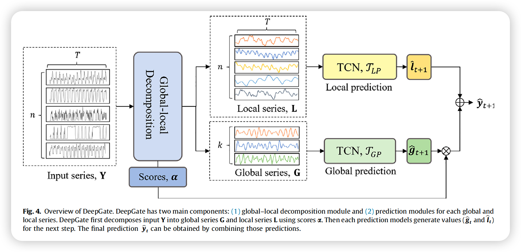
2 components :

• (1) decomposition module
• (2) prediction module

a) Decomposition module

[ Global Series ]

\(\mathbf{G}=\tanh \left(\mathcal{T}_{\mathrm{G}}(\mathbf{Y})\right)\).

• model : TCN ( = \(\mathcal{T}_{G}\) , with parameter \(\Theta\) )
• input : entire \(n\) time series \(\left(\mathbf{Y} \in \mathbb{R}^{n \times T}\right)\)
  • ( since the model has to capture “SHARED info” across multiple TS )
• activaiton function : tanh
  • \(\mathbf{g}^{(i)}\) ranges to \((-1,1)\) , for \(i = 1, \cdots k\)

[ Global Score ]

compute \(\boldsymbol{\alpha}\) from the free parameters \(\mathbf{S} \in \mathbb{R}^{n \times k}\) using the softmax operation

• \(\alpha_{i j}=\operatorname{softmax}\left(s_{i j}\right) =\frac{\exp \left(s_{i j}\right)}{\sum_{h} \exp \left(s_{i h}\right)}\).
• \(\tilde{\boldsymbol{y}}^{(i)}=\sum_{j=1}^{k} \alpha_{i j} \cdot \mathbf{g}^{(j)}\).
  • where \(\sum_{j=1}^{k} \alpha_{i j}=1\)
• \(\tilde{\boldsymbol{Y}}=\boldsymbol{\alpha} \boldsymbol{G}\).
  • where \(\tilde{\boldsymbol{Y}}=\left\{\tilde{\boldsymbol{y}}^{(1)}, \tilde{\boldsymbol{y}}^{(2)}, \ldots, \tilde{\boldsymbol{y}}^{(n)}\right\}^{\top}\)

[ Local Series ]

\(\mathbf{L}=\mathbf{Y}-\boldsymbol{\alpha} \mathbf{G}\).

Dimension

• (0) \(\mathbf{Y} \in \mathbb{R}^{n \times T}\).
• (1) \(\mathbf{G} \in \mathbb{R}^{k \times T}\)
• (2) \(\mathbf{L} \in \mathbb{R}^{n \times T}\)
• (3) \(\boldsymbol{\alpha} \in \mathbb{R}^{n \times k}\)

b) Prediction module

from decomposition module, obtain…

• \(\mathbf{G} \in \mathbb{R}^{k \times T}\), \(\mathbf{L} \in \mathbb{R}^{n \times T}\), \(\boldsymbol{\alpha} \in \mathbb{R}^{n \times k}\)

now, generate forecast!

( separate prediction layers for Global & Local )

[ Global Prediction Network ]

• (input) Global Series : \(\mathbf{G}\)
• (output) Global Prediction : \(\widehat{\mathbf{g}}_{t}=\tanh \left(\mathcal{T}_{G P}(\mathbf{G})\right)\) …… for the next time step
  • \(\mathcal{T}_{G P}\) = TCN

[ Local Prediction Network ]

• (input) Local Series : \(\mathbf{L}\)

• (output) Local Prediction ( for EACH time series ) : \(\widehat{\boldsymbol{l}}_{t} \in \mathbb{R}^{n \times 1}\)

  • \(\widehat{l}_{t}^{(i)}=\mathcal{T}_{L P}\left(\mathbf{Z}^{(i)}\right)\).

    • where \(\tilde{Z}^{(i)}=\left[\boldsymbol{l}^{(i)} ; \mathbf{Z}\right]\)

      ( \(\tilde{\boldsymbol{Z}}^{(i)}=\left[\boldsymbol{l}^{(i)} ; \boldsymbol{Z}\right] \in \mathbb{R}^{(1+\mathrm{r}) \times \mathrm{T}}\) )

  • \(\mathcal{T}_{L P}\) = TCN

• (NOTE) does not have tanh

[ Final Prediction ]

\(\widehat{\boldsymbol{y}}_{t}=\widehat{\boldsymbol{l}}_{t}+\boldsymbol{\alpha} \cdot \widehat{\boldsymbol{g}}_{t}\).

(4) Denoting training technique

Rolling Forecast

• use teacher forcing : cause a discrepancy between “train & inference”
• Causes an EXPOSURE BIAS

To alleviate this, consider simple denoising training technique for MTS forecasting

• model should be prepared for contaminated predictions

\(\rightarrow\) add noise into the inputs for the model!

\(Y^{\prime}=\boldsymbol{Y}+\gamma \cdot \varepsilon \cdot \sigma(\boldsymbol{Y}), \varepsilon \sim N(0,1)\).

• \(\sigma(\mathbf{Y})\) : empirical std
• randomly mask 50% of inputs to add noise!
• use noisy input “ONLY in the TRAIN steps”

(5) Training method

To assure the goal of “global series estimation”,

\(\rightarrow\) encouragfe the global series to have information to represent original TS

\(\rightarrow\) reconstruction loss between \(Y\) & \(\alpha G\)

( but, allow differences, for the space for “local TS” )

\(\mathcal{L}_{R}=\mathcal{L}_{1}(\mathbf{Y}, \boldsymbol{\alpha} \mathbf{G})+\lambda \mathcal{R}(\mathbf{S})\).