( reference : Machine Learning Data Lifecycle in Production )
Feature Engineering with TFX
Goal : building a DATA PIPELINE using Tensorflow Extended (TFX)
Dataset : Metro Interstate Traffic Volume dataset
Details
- create an Interactive Context to run TFX components
-
use TFX ExampleGen to split dataset
- use TFX StatisticsGen & TFX SchemaGen to generate stat & schema
- use TFX ExampleValidator to validate evaluation dataset statistics
- use TFX Transform to perform feature engineering
Contents
- Setup
- import & define paths
- EDA
- create Interactive context
- TFX components
ExampleGenStatisticsGenSchemaGenExampleValidatorTransform
- Result
1. Setup
(1) import & define paths
설치 ( 반드시 런타임 재실행 할 것! )
!pip install -U tfx
불러올 (메인) 패키지 : tf & tfx
import tensorflow as tf

import tfx
from tfx.components import (CsvExampleGen, ExampleValidator, SchemaGen, StatisticsGen, Transform)
from tfx.orchestration.experimental.interactive.interactive_context import InteractiveContext
from google.protobuf.json_format import MessageToDict

import os
import pprint

pp = pprint.PrettyPrinter()
각종 경로
# pipeline metadata store
_pipeline_root = 'metro_traffic_pipeline/'

# Raw data
_data_root = 'metro_traffic_pipeline/data'

# Raw training data
_data_filepath = os.path.join(_data_root, 'metro_traffic_volume.csv')
데이터 간단 소개
- hourly traffic volume of a road in Minnesota from 2012-2018
- goal : predicting the traffic volume given the date, time, and weather conditions
(3) create Interactive context
initialize InteractiveContext
context = InteractiveContext(pipeline_root=_pipeline_root)
2. TFX components
(1) ExampleGen
Summary ( = Ingesting Data )
- (1) split data ( train 2/3 : eval 1/3 )
- (2) convert each row into
tf.train.Exampleformat - (3) compress & save data, under
_pipeline_rootdir- reason : for other components to access!
- stored in
TFRecordformat
Example 1) ingest csv data
( = run the component, using InteractiveContext instance )
example_gen = CsvExampleGen(input_base=_data_root)
context.run(example_gen)
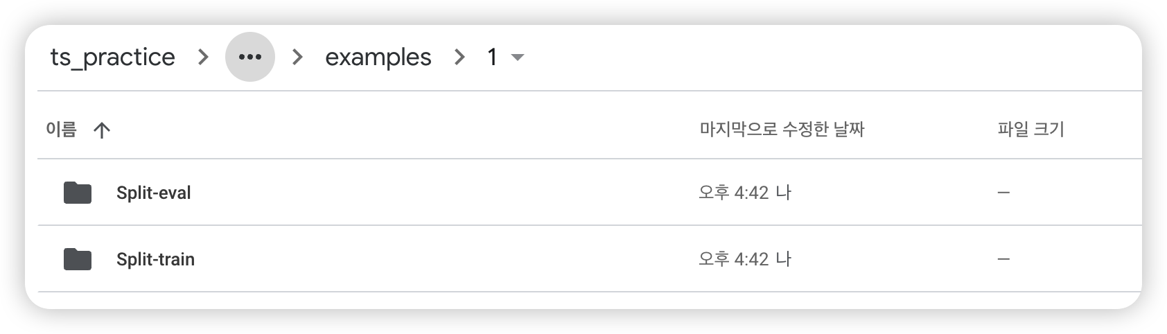
위와 같이, 데이터셋이 나눠진 것을 확인할 수 있다
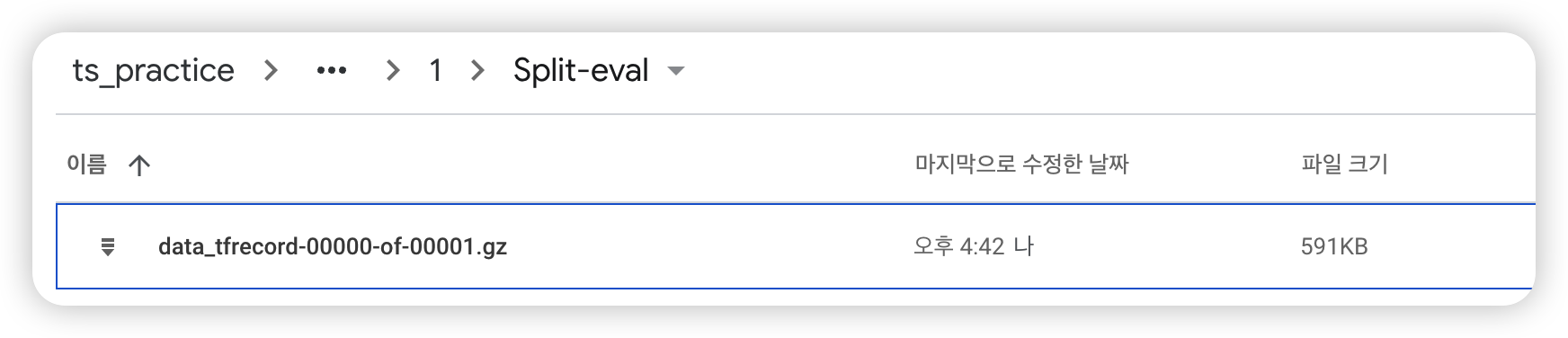
잘 생성되었나 확인 가능
# context.run() 작동 O 경우 ( = interactive )
try:
artifact = example_gen.outputs['examples'].get()[0]
print(f'split names: {artifact.split_names}')
print(f'artifact uri: {artifact.uri}')
# context.run() 작동 X 경우 ( = non-interactive )
except IndexError:
print("context.run() was no-op")
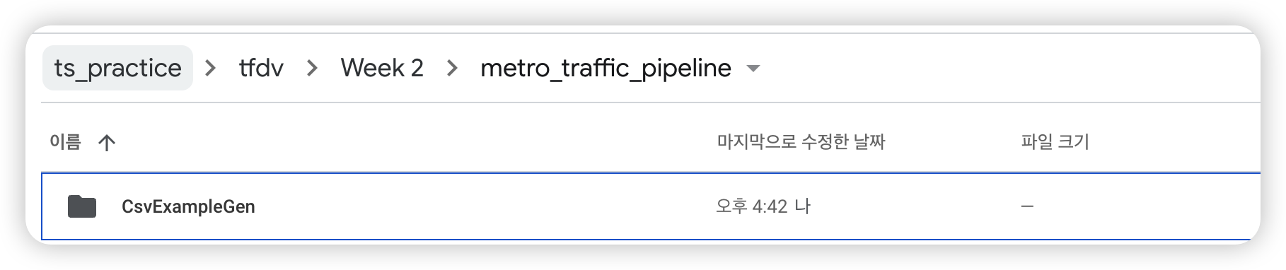
examples_path = './metro_traffic_pipeline/CsvExampleGen/examples'
dir_id = os.listdir(examples_path)[0]
artifact_uri = f'{examples_path}/{dir_id}'
else:
artifact_uri = artifact.uri
split names: ["train", "eval"]
artifact uri: metro_traffic_pipeline/CsvExampleGen/examples/1
데이터 몇 개만 확인해보자!
- URI : Uniform Resource identifier ( 여기서는, 데이터 저장 경로 )
# (1) URI ( = directory )
train_uri = os.path.join(artifact_uri, 'Split-train')

# (2) URL 내의 파일명들
tfrecord_filenames = [os.path.join(train_uri, name)
                      for name in os.listdir(train_uri)]

# (3) `TFRecordDataset`를 사용하여 위 파일들을 불러옴
dataset = tf.data.TFRecordDataset(tfrecord_filenames, compression_type="GZIP")
Example 2) ingest csv data
지정한 개수 만큼의 example을 가져와보자. ( 함수 : get_records() )
get_records(dataset, num_records)
- dataset :
TfRecordDataset포맷
def get_records(dataset, num_records):
    records = []

    for tfrecord in dataset.take(num_records):
        # (1) tf.train.Example() = 데이터 읽어들이기 위해
        example = tf.train.Example()

        # (2) np.array 로 변환 후, 읽어들이기
        tfrecord_np = tfrecord.numpy()

        # (3) protocol buffer message형식
        example.ParseFromString(tfrecord_np)

        # (4) protocol buffer message -> dictionary 변환
        example_dict = MessageToDict(example)
        records.append(example_dict)

    return records
결과 ( 3개의 데이터 예시를 가져옴 ) :
sample_records = get_records(dataset, 3)
pp.pprint(sample_records)
[{'features': {'feature': {'clouds_all': {'int64List': {'value': ['40']}},
                           'date_time': {'bytesList': {'value': ['MjAxMi0xMC0wMiAwOTowMDowMA==']}},
                           'day': {'int64List': {'value': ['2']}},
                           'day_of_week': {'int64List': {'value': ['1']}},
                           'holiday': {'bytesList': {'value': ['Tm9uZQ==']}},
                           'hour': {'int64List': {'value': ['9']}},
                           'month': {'int64List': {'value': ['10']}},
                           'rain_1h': {'floatList': {'value': [0.0]}},
                           'snow_1h': {'floatList': {'value': [0.0]}},
                           'temp': {'floatList': {'value': [288.28]}},
                           'traffic_volume': {'int64List': {'value': ['5545']}},
                           'weather_description': {'bytesList': {'value': ['c2NhdHRlcmVkIGNsb3Vkcw==']}},
                           'weather_main': {'bytesList': {'value': ['Q2xvdWRz']}}}}},
 {'features': {'feature': {'clouds_all': {'int64List': {'value': ['75']}},
                           'date_time': {'bytesList': {'value': ['MjAxMi0xMC0wMiAxMDowMDowMA==']}},
                           'day': {'int64List': {'value': ['2']}},
                           'day_of_week': {'int64List': {'value': ['1']}},
                           'holiday': {'bytesList': {'value': ['Tm9uZQ==']}},
                           'hour': {'int64List': {'value': ['10']}},
                           'month': {'int64List': {'value': ['10']}},
                           'rain_1h': {'floatList': {'value': [0.0]}},
                           'snow_1h': {'floatList': {'value': [0.0]}},
                           'temp': {'floatList': {'value': [289.36]}},
                           'traffic_volume': {'int64List': {'value': ['4516']}},
                           'weather_description': {'bytesList': {'value': ['YnJva2VuIGNsb3Vkcw==']}},
                           'weather_main': {'bytesList': {'value': ['Q2xvdWRz']}}}}},
 {'features': {'feature': {'clouds_all': {'int64List': {'value': ['90']}},
                           'date_time': {'bytesList': {'value': ['MjAxMi0xMC0wMiAxMTowMDowMA==']}},
                           'day': {'int64List': {'value': ['2']}},
                           'day_of_week': {'int64List': {'value': ['1']}},
                           'holiday': {'bytesList': {'value': ['Tm9uZQ==']}},
                           'hour': {'int64List': {'value': ['11']}},
                           'month': {'int64List': {'value': ['10']}},
                           'rain_1h': {'floatList': {'value': [0.0]}},
                           'snow_1h': {'floatList': {'value': [0.0]}},
                           'temp': {'floatList': {'value': [289.58]}},
                           'traffic_volume': {'int64List': {'value': ['4767']}},
                           'weather_description': {'bytesList': {'value': ['b3ZlcmNhc3QgY2xvdWRz']}},
                           'weather_main': {'bytesList': {'value': ['Q2xvdWRz']}}}}}]
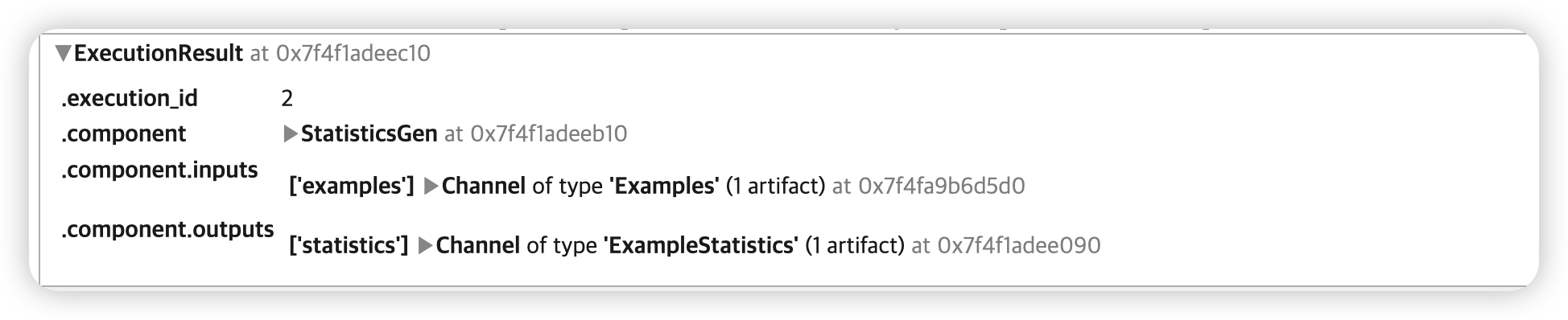
(2)StatisticsGen
-
데이터셋에 대한 statistcis를 계산하기 위함
-
TensorFlow Data Validaiton사용
# StatisticsGen를 인스턴스화
# ( 위에서 만든 ingested dataset을 사용하여 )
statistics_gen = StatisticsGen(examples=example_gen.outputs['examples'])
context.run(statistics_gen)
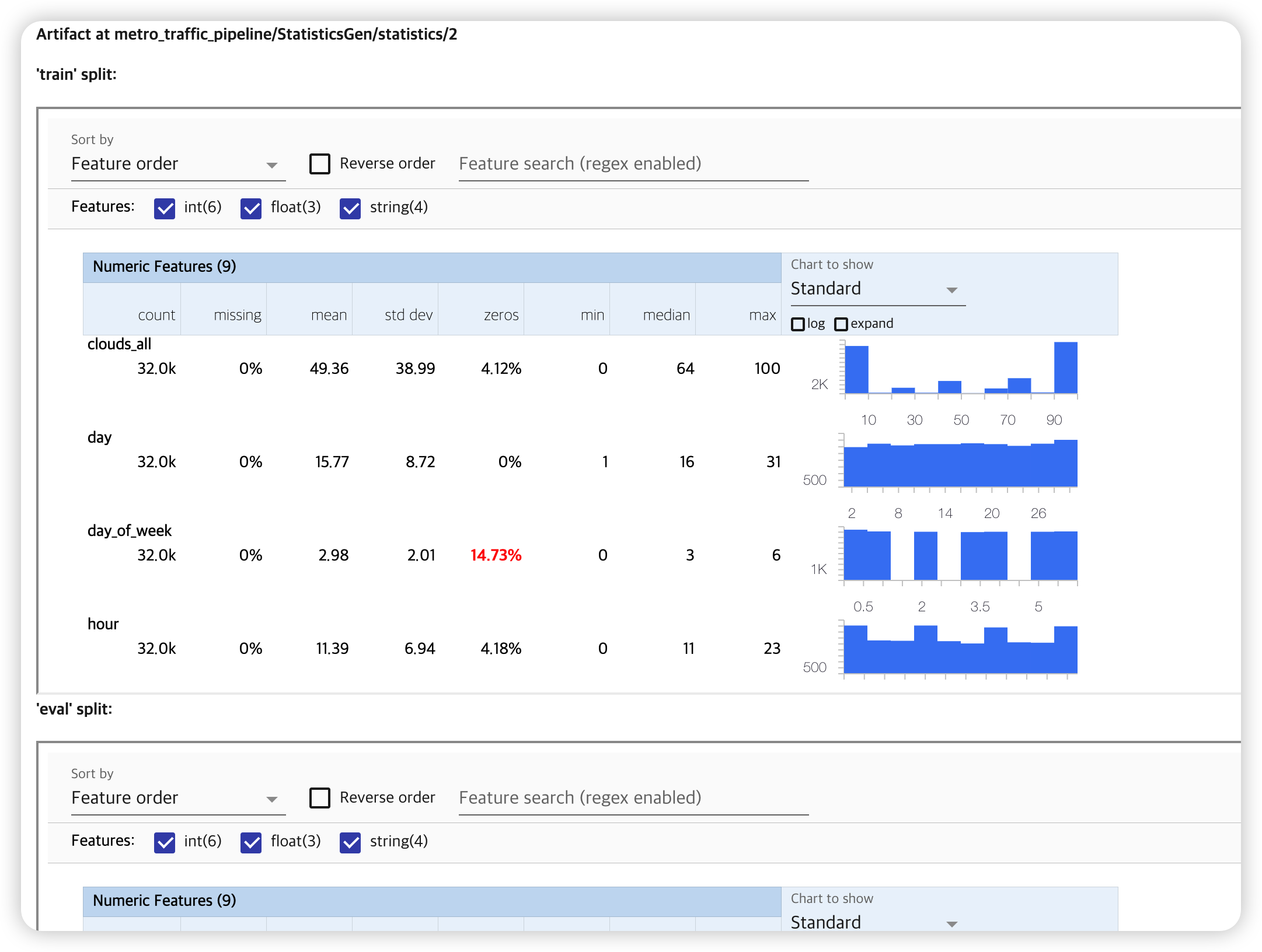
생성한 statistic을 시각적으로 확인해보자.
context.show(statistics_gen.outputs['statistics'])
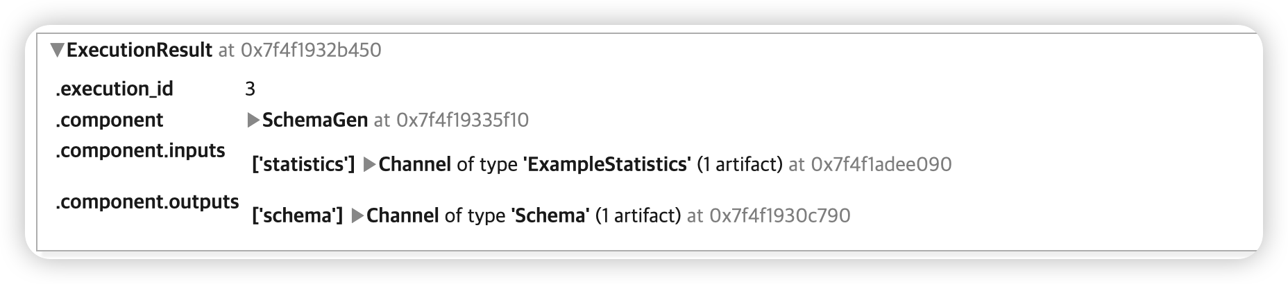
(3) SchemaGen
- 위에서 생성한 statistics를 바탕으로 schema 생성하기 위함
- 스키마 : expected bounds, types, properties of features
TensorFlow Data Validaiton사용
# SchemaGen를 인스턴스화
# ( 위에서 만든 statistics을 사용하여 )
schema_gen = SchemaGen(statistics=statistics_gen.outputs['statistics'])
context.run(schema_gen)
생성한 schema를 시각적으로 확인해보자
context.show(schema_gen.outputs['schema'])
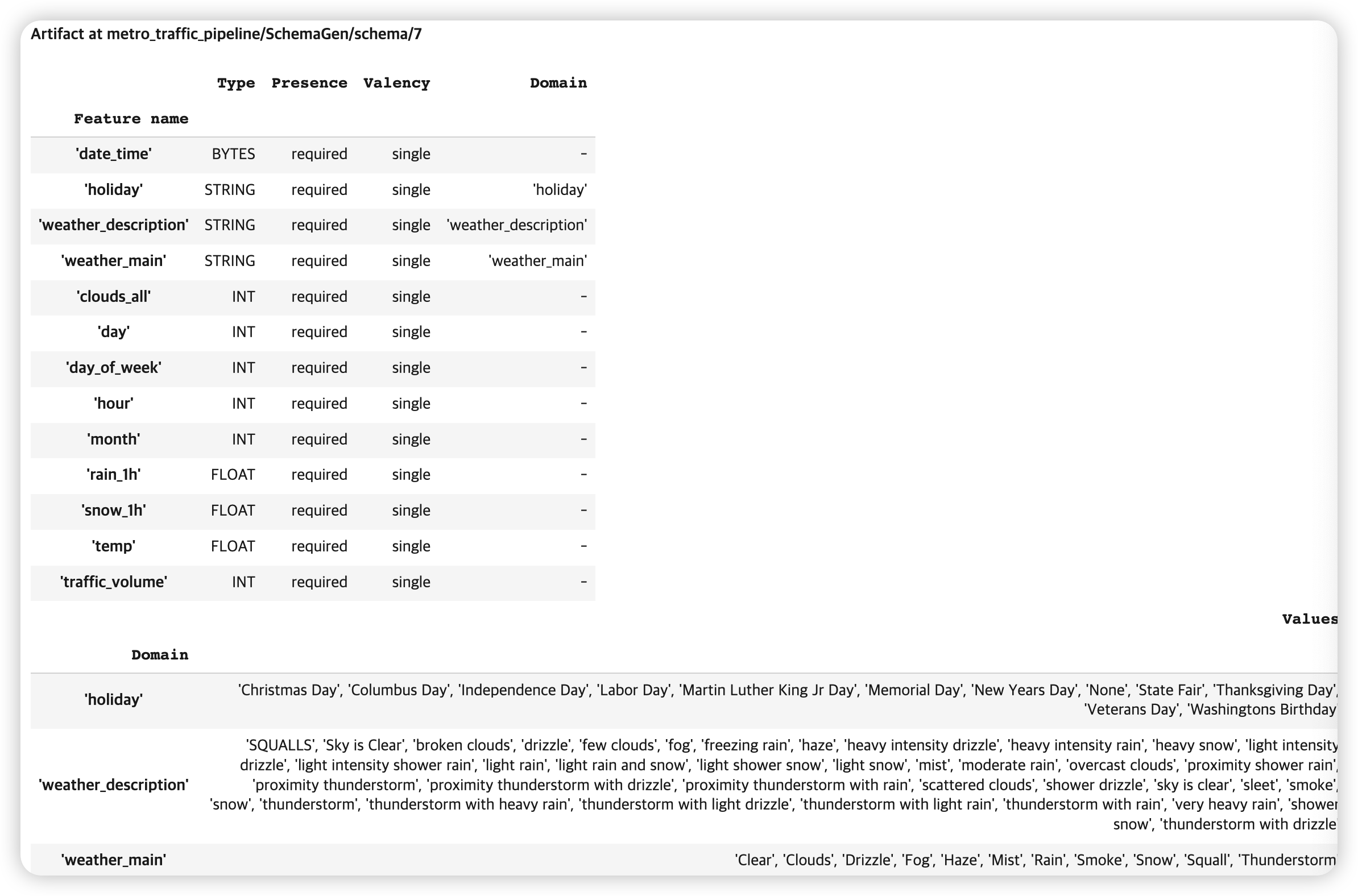
이렇게 생성한 schema는, 뒤에서 anomaly를 detect 하는데에 활용된다.
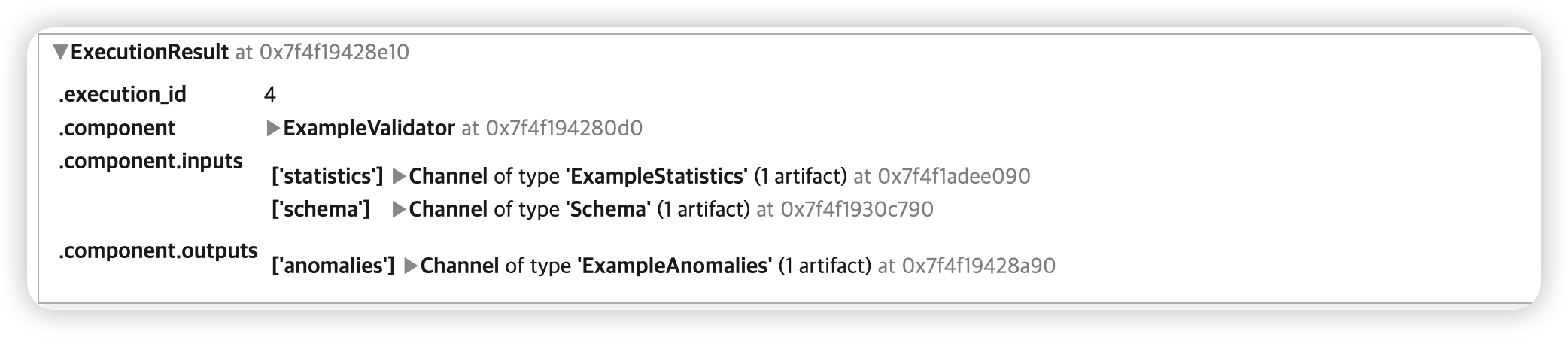
(4) ExampleValidator
- 위에서 생성한 schema & statistics를 바탕으로, anomaly를 detect하는데에 사용된다.
TensorFlow Data Validaiton사용- (default로) training & evaluation split을 비교한다
example_validator = ExampleValidator(statistics = statistics_gen.outputs['statistics'],
                                     schema = schema_gen.outputs['schema'])

context.run(example_validator)
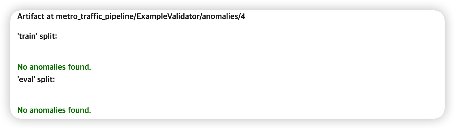
detect한 anomaly들을 시각적으로 확인해보자
context.show(example_validator.outputs['anomalies'])
(5) Transform
- 위에서 생성한 examplegen & statistics를 바탕으로, feature engineering을 하기 위함
- 수행하고자 하는 “전처리 함수” 또한 필요함
- magic command
%% writefile을 사용하여, 전처리 함수 코드를 저장한다!
(1) 저장할 이름
_traffic_constants_module_file = 'traffic_constants.py'
(2) 변환 대상 & 함수 정의 ( _traffic_constants_module_file )
%%writefile {_traffic_constants_module_file}

# (1)z-score 정규화할 변수
DENSE_FLOAT_FEATURE_KEYS = ['temp', 'snow_1h']

# (2) bucketize 할 변수 & bucket 개수
BUCKET_FEATURE_KEYS = ['rain_1h']
FEATURE_BUCKET_COUNT = {'rain_1h': 3}

# (3) 0~1 스케일링할 변수
RANGE_FEATURE_KEYS = ['clouds_all']

# (4) vocabulary 개수 & oov 기준 개수
VOCAB_SIZE = 1000
OOV_SIZE = 10

# (5) string -> indicies 변환할 변수
VOCAB_FEATURE_KEYS = [
    'holiday',
    'weather_main',
    'weather_description'
]

# (6) (int형으로 된) 범주형 변수 ( 그대로 유지 )
CATEGORICAL_FEATURE_KEYS = [
    'hour', 'day', 'day_of_week', 'month'
]

# (7) 타겟 변수
VOLUME_KEY = 'traffic_volume'

def transformed_name(key):
    return key + '_xf'
(3) 저장할 이름
_traffic_transform_module_file = 'traffic_transform.py'
(4) 전처리 수행
%%writefile {_traffic_transform_module_file}

import tensorflow as tf
import tensorflow_transform as tft

import traffic_constants

# constants module으 내용들 unpack
_DENSE_FLOAT_FEATURE_KEYS = traffic_constants.DENSE_FLOAT_FEATURE_KEYS
_RANGE_FEATURE_KEYS = traffic_constants.RANGE_FEATURE_KEYS
_VOCAB_FEATURE_KEYS = traffic_constants.VOCAB_FEATURE_KEYS
_VOCAB_SIZE = traffic_constants.VOCAB_SIZE
_OOV_SIZE = traffic_constants.OOV_SIZE
_CATEGORICAL_FEATURE_KEYS = traffic_constants.CATEGORICAL_FEATURE_KEYS
_BUCKET_FEATURE_KEYS = traffic_constants.BUCKET_FEATURE_KEYS
_FEATURE_BUCKET_COUNT = traffic_constants.FEATURE_BUCKET_COUNT
_VOLUME_KEY = traffic_constants.VOLUME_KEY
_transformed_name = traffic_constants.transformed_name


def preprocessing_fn(inputs):
    #-------------------------------------------------#
    # dictionary 형태의 INPUT & OUTPUT
    outputs = {}
    #-------------------------------------------------#
    # (1) 전처리 1
    for key in _DENSE_FLOAT_FEATURE_KEYS:
        outputs[_transformed_name(key)] = tft.scale_to_z_score(inputs[key])

	  # (2) 전처리 2
    for key in _RANGE_FEATURE_KEYS:
        outputs[_transformed_name(key)] = tft.scale_to_0_1(inputs[key])

    # (3) 전처리 3
    for key in _VOCAB_FEATURE_KEYS:
        outputs[_transformed_name(key)] = tft.compute_and_apply_vocabulary(
            inputs[key],
            top_k=_VOCAB_SIZE,
            num_oov_buckets=_OOV_SIZE)

    # (4) 전처리 4
    for key in _BUCKET_FEATURE_KEYS:
        outputs[_transformed_name(key)] = tft.bucketize(
            inputs[key],
            _FEATURE_BUCKET_COUNT[key])

    # (5) 전처리 5
    for key in _CATEGORICAL_FEATURE_KEYS:
        outputs[_transformed_name(key)] = inputs[key]


    # target value에서 결측치 채우기 & float32로 형식 바꾸기 & binary 형식으로
    ## ( 결측치 채우는 함수는 아래 참고 )
    traffic_volume = tf.cast(_fill_in_missing(inputs[_VOLUME_KEY]), tf.float32)

    outputs[_transformed_name(_VOLUME_KEY)] = tf.cast(
        tf.greater(traffic_volume,
                   tft.mean(tf.cast(traffic_volume, tf.float32))),tf.int64)


    return outputs


def _fill_in_missing(x):
    if not isinstance(x, tf.sparse.SparseTensor):
      return x

    default_value = '' if x.dtype == tf.string else 0
    return tf.squeeze(
        tf.sparse.to_dense(
            tf.SparseTensor(x.indices, x.values, [x.dense_shape[0], 1]),
            default_value),
        axis=1)
Feature Engineering 하기
# to ignore tf warning
tf.get_logger().setLevel('ERROR')


# Transform component를 인스턴스화
## 구성요소 3개
transform = Transform(
    examples = example_gen.outputs['examples'],
    schema = schema_gen.outputs['schema'],
    module_file = os.path.abspath(_traffic_transform_module_file))

context.run(transform)
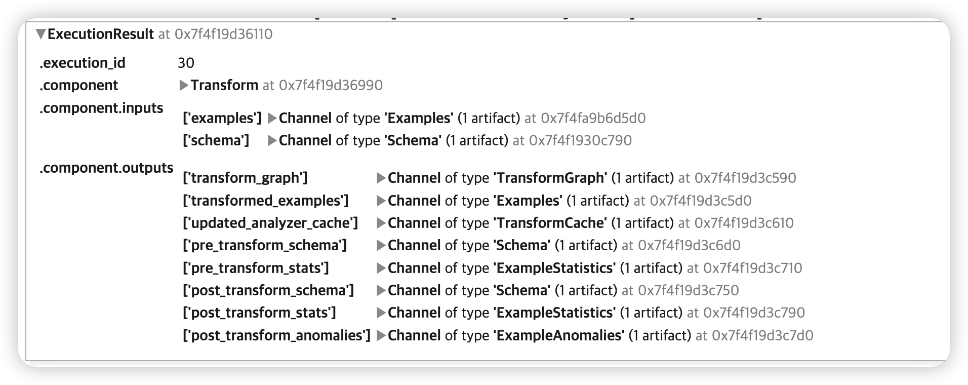
3. Result
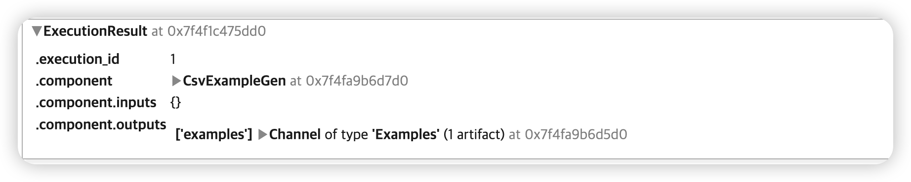
위의 InteractiveContext의 output cell을, .component.outputs 에서 확인할 수 있다.
transform_graph: preprocessing을 수행하는 그래프- training & serving에서 둘 다 사용될 것
transformed_examples: preprocessed training & evaluation data
Transform Graph의 URI 가져오기
try:
    transform_graph_uri = transform.outputs['transform_graph'].get()[0].uri

except IndexError:
    print("context.run() was no-op")
    transform_path = './metro_traffic_pipeline/Transform/transformed_examples'
    dir_id = os.listdir(transform_path)[0]
    transform_graph_uri = f'{transform_path}/{dir_id}'

else:
    os.listdir(transform_graph_uri)
Transform된 training data의 URI 가져오기
try:
    train_uri = os.path.join(transform.outputs['transformed_examples'].get()[0].uri,
                             'train')

except IndexError:
    print("context.run() was no-op")
    train_uri = os.path.join(transform_graph_uri, 'train')
tfrecord_filenames = [os.path.join(train_uri, name)
                      for name in os.listdir(train_uri)]

transformed_dataset = tf.data.TFRecordDataset(tfrecord_filenames,
                                              compression_type="GZIP")
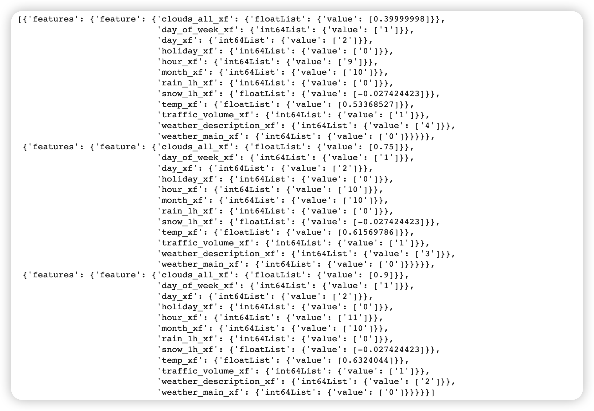
transform이 완료된 데이터 상위 3개 가져오기
sample_records_xf = get_records(transformed_dataset, 3)

pp.pprint(sample_records_xf)