
Gradient Boosting Neural Networks: GrowNet
https://arxiv.org/abs/2002.07971
Contents
- Abstract
- Introduction
- Model
- GrowNet
- Corrective Step
- Application
- Regression: MSE loss
- Classification: BCE loss
Abstract
Grownet
- gradient boosting ( multiple shallow models ) + NN
- outperform SOTA boosting methods in 3 tasks on multiple datasets
1. Introduuction
DT vs DNN
- DT) not unversally applicable ( ex. NLP, CV )
- DNN) perform much better
GrowNet
-
builds NN from the ground up layer by layer
( + with idea of gradient boosting )
2. Model
Key Idea of gradient boosting : simple, lower-order models
- use shallow NN
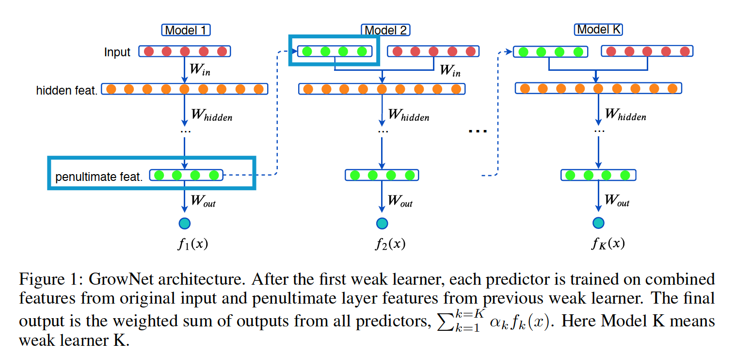
As each boosting step, augment original input features with the output from the penultimate layer of the current iteration.
(1) Gradient Boosting NN: GrowNet
Dataset : \(\mathcal{D}=\left\{\left(\boldsymbol{x}_i, y_i\right)_{i=1}^n \mid \boldsymbol{x}_i \in\right.\) \(\left.\mathbb{R}^d, y_i \in \mathbb{R}\right\}\).
Prediction :\(K\) additive functions
-
\[\hat{y}_i=\mathcal{E}(\boldsymbol{x}_i)=\sum_{k=0}^K \alpha_k f_k(\boldsymbol{x}_i)\]
- weighted sum of \(f_k\) ‘s in GrowNet.
- \(f_k \in \mathcal{F}\), where \(\mathcal{F}\) is the space of MLP
- \(\alpha_k\) : the step size (boost rate).
- Each function \(f_k\) represents an independent, shallow NN
Loss Function: \(\mathcal{L}(\mathcal{E})=\sum_{i=0}^n l\left(y_i, \hat{y}_i\right)\).
Greedy search
-
\(\hat{y}_i^{(t-1)}=\sum_{k=0}^{t-1} \alpha_k f_k\left(\boldsymbol{x}_i\right)\) : output of GrowNet at stage \(t-1\) for the sample \(\boldsymbol{x}_i\).
-
greedily seek the next weak learner \(f_t(\mathbf{x})\) that will minimize the loss at stage \(t\)
- \(\mathcal{L}^{(t)}=\sum_{i=0}^n l\left(y_i, \hat{y}_i^{(t-1)}+\alpha_t f_t\left(\mathbf{x}_i\right)\right)\).
Taylor expansion of the loss function \(l\)
-
to ease the computational complexity.
-
objective function for the weak learner \(f_t\) can be simplified as..
\(\mathcal{L}^{(t)}=\sum_{i=0}^n h_i\left(\tilde{y}_i-\alpha_t f_t\left(\boldsymbol{x}_i\right)\right)^2\).
- where \(\tilde{y}_i=-g_i / h_i\)
- \(g_i\) : second order gradients of \(l\) at \(\boldsymbol{x}_i\), w.r.t. \(\hat{y}_i^{(t-1)}\)
- \(h_i\) : second order gradients of \(l\) at \(\boldsymbol{x}_i\), w.r.t. \(\hat{y}_i^{(t-1)}\)
- where \(\tilde{y}_i=-g_i / h_i\)
(2) Corrective Step (C/S)
Traditional boosting : each weak learner is greedily learned
\(\rightarrow\) local minimia ( + due to fixed boosting rate \(\alpha_k\) )
Solution: corrective step
\(\rightarrow\) instead of fixing the previous \(t-1\) weak learners…
update the parameters of ALL previous \(t-1\) weak learners!
3. Application
Regression & Classifcation & Learning to Rank
(1) Regression: MSE loss
- \(g_i=2\left(\hat{y}_i^{(t-1)}-y_i\right)\);
- \(h_i=2\).
- \(\tilde{y}_i=y_i-\hat{y}_i^{(t-1)}\).
Train next weak learner \(f_t\) by least square regression on \(\left\{\boldsymbol{x}_i, \tilde{y}_i\right\}\) for \(i=1,2, \ldots, n\).
(2) Classification: BCE loss
- \(g_i=\frac{-2 y_i}{1+e^{2 y_i \hat{y}_i^{(t-1)}}}\).
- \(h_i=\frac{4 y_i^2 e^{2 y_i \hat{y}_i^{(t-1)}}}{\left(1+e^{2 y_i \hat{y}_i^{(t-1)}}\right)^2}\).
- \(\tilde{y}_i=-g_i / h_i=y_i\left(1+e^{-2 y_i \hat{y}_i^{(t-1)}}\right) / 2\).