Learning Problem-agnostic Speech Representations from Multiple Self-supervised Tasks

Learning Problem-agnostic Speech Representations from Multiple Self-supervised Tasks ( arxiv 2019 )

https://arxiv.org/pdf/1904.03416.pdf

Contents

1. Abstract
2. Introduction
3. PASE (Problem-agnostic Speech Encoder)
   1. Encoder
   2. Workers
   3. Self-supervised Training
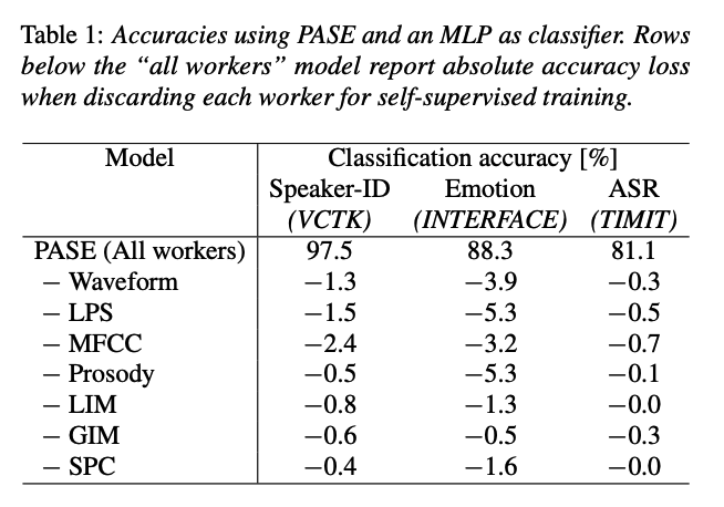
4. Ablation study of workers

Abstract

PASE: self supervised method

• single encoder is followed by multiple workers
  • multiple workers = jointly solve different self-supervised tasks

Experiments

• carry on relevant information from the speech signal, such as speaker identity, phonemes, and even higher-level features such as emotional cues.

1. Introduction

Challenges of speech signals

• high-dimensional, long, and variable-length sequences
• entail a complex hierarchical structure
  • that is difficult to infer without supervision (phonemes, syllables, words, etc.).
• Thus hard to find a single self-supervised task that can learn general and meaningful representations able to capture this latent structure.

Solution : propose to jointly tackle multiple self-supervised tasks using an ensemble of neural networks

• intuition : each self-supervised task may bring a different view or soft constraint on the learned representation.
• requires consensus across tasks, imposing several constraints into the learned representations.

\(\rightarrow\) proposed architecture = problem-agnostic speech encoder (PASE)

• encodes the raw speech waveform into a representation
• fed to multiple regressors and discriminators ( = workers )
  • Regressors = deal with standard features computed from the input waveform
    • resemble a decomposition of the signal at many levels.
  • Discriminators = deal with either positive or negative samples
    • trained to separate them by minimizing BCE loss

2. PASE (Problem-agnostic Speech Encoder)

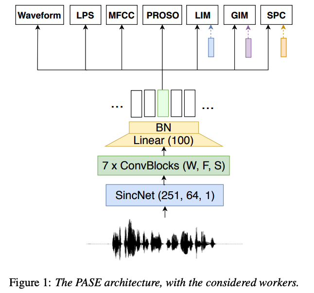
PASE architecture

• (1) fully-convolutional speech encoder
• (2) 7 multilayer perceptron (MLP) workers

(1) Encoder

a) 1st layer = SincNet model

• performs the convolution of the raw input waveform with a set of parameterized sinc functions that implement rectangular band-pass filters.
• interesting property = the number of parameters does not increase with the kernel size
  • use a large kernel width \(W=251\) to implement \(F=64\) filters with a stride \(S=1\).

b) 2nd layers = stack of 7 convolutional blocks

• each block employs a 1D convolution, followed by BN
• multi-parametric rectified linear unit (PReLU) activation
• details (of 7 blocks)
  • kernel widths \(W=\{20,11,11,11,11,11,11\}\)
  • filters \(F={64,128,128,256,256,512,512}\)
  • strides \(S=\) \(\{10,2,1,2,1,2,2\}\).

c) 3rd layer = convolution with \(W=1\)

• projects 512 features to embeddings of 100 dim
• non-affine BN layer

(2) Workers

7 self-supervised tasks

• regression or binary discrimination tasks

• workers are based on very small feed-forward networks

  • composed of a single hidden layer of 256 units with PReLU activation

    (the only exception is the waveform worker, see below).

• encourage the encoders to discover high-level features

Regression workers

• break down the signal components at many levels in an increasing order of abstraction

• trained to minimize MSE

  (again the waveform worker is an exception)

4 Regression workers

• (1) Waveform
  • predict the input waveform in an auto-encoder fashion
  • (exception) Decoder
    • Three deconvolutional blocks
      • with strides 4,4 , and 10 that upsample the encoder representation by a factor of 160
    • MLP of 256 PReLU units is used with a single output unit per timestep.
  • (exception) minimize MAE
    • Why MAE? as the speech distribution is very peaky and zero-centered with prominent outliers
• (2) Log power spectrum (LPS)
  • compute it using a Hamming window of \(25 \mathrm{~ms}\) and a step size of \(10 \mathrm{~ms}\), with 1025 frequency bins per time step.
• (3) Mel-frequency cepstral coefficients (MFCC)
  • extract 20 coefficients from 40 mel filter banks (FBANKs).
• (4) Prosody
  • predict four basic features per frame, namely the interpolated logarithm of the fundamental frequency, voiced/unvoiced probability, zero-crossing rate, and energy ( = called “Prosody” )

Discrimination workers

• 3 binary discrimination tasks
  • learning a higher level of abstraction than that of signal features
• rely on a pre-defined sampling strategy
  • draws an anchor \(x_a\), a positive \(x_p\), and a negative \(x_n\) sample from the pool of PASE-encoded representations
    • reference \(x_a\) = an encoded feature extracted from a random sentence
    • negative & positive = drawn using the different sampling strategies described below
• Loss function :
  • \(L=\mathbb{E}_{X_p}\left[\log \left(g\left(x_a, x_p\right)\right)\right]+\mathbb{E}_{X_n}\left[\log \left(1-g\left(x_a, x_n\right)\right)\right]\).
    • where \(g\) is the discriminator function
• Notice that the encoder and the discriminators are not adversarial here, but must cooperate!

Sampling POS & NEG

• Local info max (LIM)
• Global info max (GIM)
• Sequence predicting coding (SPC)

(3) Self-supervised Training

Encoder and workers

• jointly trained with backpropagation
• total loss = average of each worker cost

Gradients of encoder

• gradient coming from the workers are thus averaged

To balance the contribution of each regression loss….

• we standardize all worker outputs, before computing the MSE

3. Ablation study of workers