Unsupervised Contrastive Learning of Sound Event Representations

Unsupervised Contrastive Learning of Sound Event Representations (arXiv, 2020)

https://arxiv.org/pdf/2011.07616.pdf

Contents

1. Abstract
2. Introduction
3. Method
   1. Stochastic sampling of data views
   2. Mix-back
   3. Stochastic Data Augmentation
   4. Architectures

Abstract

Unsupervised contrastive learning as a way to learn sound event representations

Propose to use the pretext task of contrasting differently augmented views of sound events

• views are computed primarily via mixing of training examples with unrelated backgrounds,

  followed by other data augmentations.

1. Introduction

Sound event recognition (SER)

Two largest labeled SER datasets

• (1) AudioSet
  • provides a massive amount of content but the official release does not include waveforms, and the labelling in some classes is less precise
• (2) FSD50K
  • consists of open-licensed audio curated with a more thorough labeling process,
  • but the data amount is more limited.

Related works in SSL

(1) First works in SSL sound event representation learning [7]

• adopting a triplet loss-based training by creating anchor-positive pairs via simple audio transformations
  • e.g., adding noise or mixing examples.

(2) Predicting the long-term temporal structure of continuous recordings captured with an acoustic sensor network [12]

(3) Two pretext tasks [11]

• a) estimating the time distance between pairs of audio segments
• b) reconstructing a spectrogram patch from past and future patches

Proposal

pretext task of contrasting differently augmented views of sound events

• different views = via mixing of training examples with unrelated background examples, followed by other data augmentations.

Experiments

• linear evaluation
• two downstream sound event classification tasks

2. Method

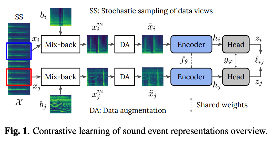
(1) Stochastic sampling of data views

• Input \(\mathcal{X}\) : log-mel spectrograms of audio clips
• Sample 2 views = time frequency (TF) patches
  • \(x_i \in \mathcal{X}\) and \(x_j \in \mathcal{X}\) are selected randomly over the length of the clip spectrogam

(2) Mix-back

Mixing the (1) incoming patch \(x_i\) with a (2) background patch, \(b_i\)

• \(x_i^m=(1-\lambda) x_i+\lambda\left[E\left(x_i\right) / E\left(b_i\right)\right] b_i\)…… Eq (1)
  • \(\lambda \sim \mathcal{U}(0, \alpha)\).
  • \(\alpha \in[0,1]\) is the mixing hyper-parameter (typically small)
  • \(E(\cdot)\) : energy of a given patch.
• Energy adjustment of Eq. 1 ensures that \(x_i\) is always dominant over \(b_i\), even if \(E\left(b_i\right)>>\) \(E\left(x_i\right)\),
  • preventing aggressive transformations that may make the pretext task too difficult

( Details: Before Eq. 1, patches are transformed to linear scale (inversion of the log in the log-mel) to allow energywise compensation, after which mix-back is applied, and then the output, \(x_i^m\), is transformed back to log scale )

Background patches \(b\)

• randomly drawn from the training set (excluding the input clip \(\mathcal{X}\) ),

• Motivation

  • (1) shared information across positives is decreased by mixing \(x_i\) and \(x_j\) with different backgrounds
  • (2) semantic information is preserved due to sound transparency (i.e., a mixture of two sound events inherits the classes of the constituents) and the fact that the positive patch is always predominant in the mixture.

Mix-back = data augmentation (?)

• yes, but we separate it from the others as it involves two input patches.

(3) Stochastic Data Augmentation

Adopt DAs directly computable over TF patches (rather than waveforms)

• simple for on-the-fly computation

Transform \(x_i^m\) into the input patch \(\tilde{x}_i\) for the encoder network.

Consider DAs both from computer vision and audio literature

• random resized cropping (RRC)
• random time/frequency shifts
• compression
• SpecAugment
• Gaussian noise addition
• Gaussian blurring.

(4) Architectures

a) Encoder

CNN based network \(f_\theta\)

• embedding \(h_i=f_\theta\left(\tilde{x}_i\right)\) from the augmented patch \(\tilde{x}_i\),

b) Projection head

Simple projection network \(g_{\varphi}\)

• consists of an MLP with one hidden layer, batchnormalization, and a ReLU

L2-normalized low-dimensional representation \(z_i\)

c) Contrastive Loss

NT-Xent loss

\(\ell_{i j}=-\log \frac{\exp \left(z_i \cdot z_j / \tau\right)}{\sum_{v=1}^{2 N} \mathbb{1}_{v \neq i} \exp \left(z_i \cdot z_v / \tau\right)}\).