Audio Self-supervised Learning: A Survey ( arxiv 2022 )

https://arxiv.org/pdf/2203.01205.pdf

https://www.researchgate.net/publication/358974871_Audio_Self-supervised_Learning_A_Survey/link/6225b0ed84ce8e5b4d0cdbf4/download

Abstract
Audio SSL
Downstream audio Tasks & Benchmarks

Abstract

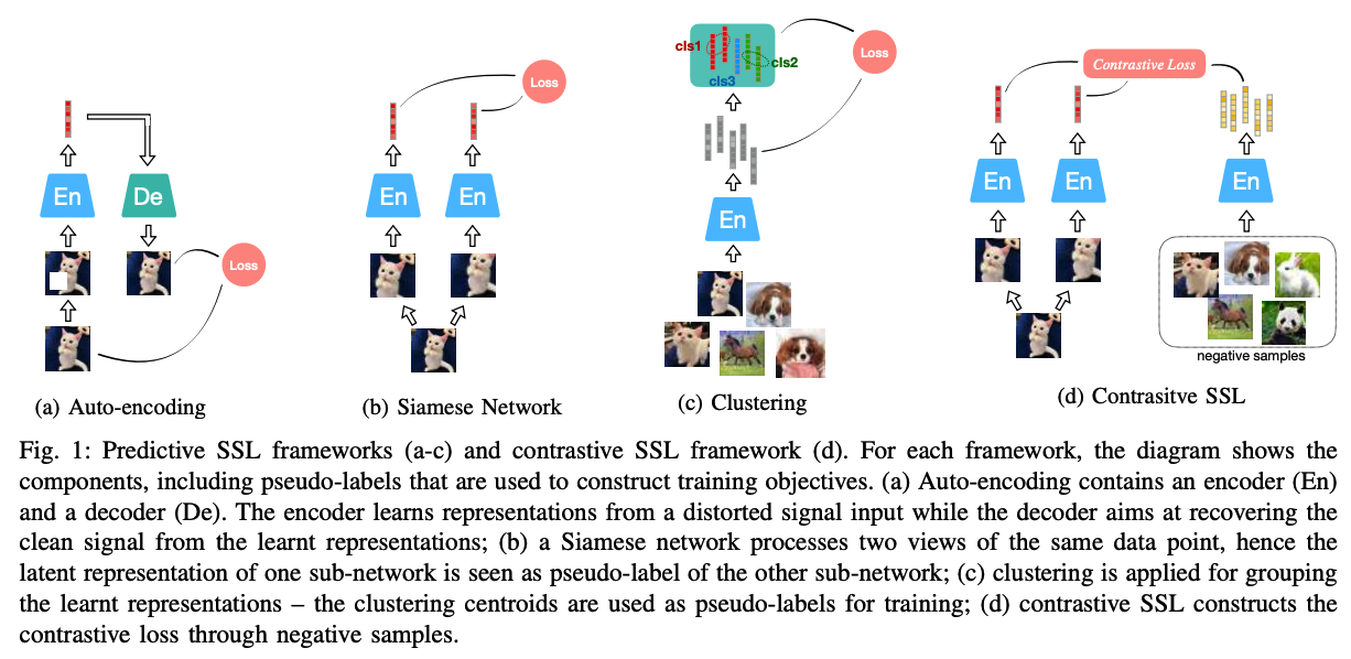
1. Self-supervised Learning: A General Overview

2. Audio SSL

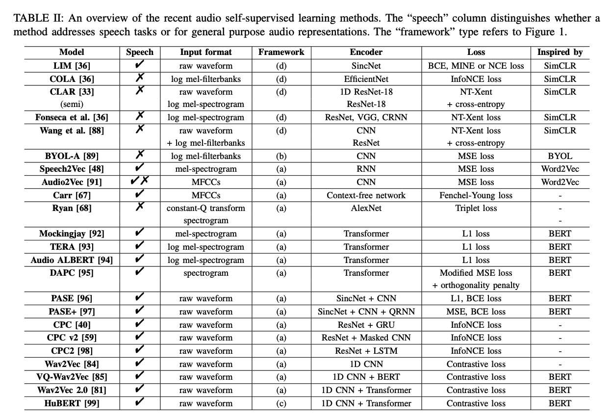
LIM [36], COLA [37], CLAR [33], Fonseca et al. [38]

expand the SimCLR approach for learning auditory representations
LIM [36]
- processes directly speech samples expecting to maximise “local mutual information” between the encoded representations of chunks of speech sampled from the same utterance
COLA [37], Fonseca et al. [38]
- take segments randomly extracted from time-frequency features along the temporal direction
- Fonseca et al. [38]
  - several stochastic data augmentations
    - ex) random size cropping and Gaussian noise addition
  - proposed “mix-back” for additional augmentation
    
    = which mixes the incoming patch with a background patch, by this ensuring that the incoming patch is dominant in their mixture.
CLAR [33]
- paired views of the model’s input
  
  = generated by applying data augmentations on raw audio signals and time frequency audio features
- combining a contrastive loss ( such as CE loss ) for supervised learning can provide significant improvements
Wang [88]
- also suggests to train audio SSL models with different formats of an audio sample
- training objective = maximise the agreement between the (1) raw waveform and its (2) spectral representation
BYOL-A [89]
- adopt BYOL in the audio domain
- learns representations from a single audio without using negative samples
Audio2Vec [49], Speech2Vec [48]
- inspired by Word2Vec [47]
- learn audio representations using CBoW and skip-gram formulations.
  - CBoW : (input, output) = (middle, past&future)
    - effective for acoustic scene classification in [90]
  - Skip-gram: (input, output) = (past&future, middle)
- Audio2Vec vs. Speech2Vec
  - (1) Audio Segmentation
    - Speech2Vec : applies audio segmentation, by using an explicit forced alignment technique
      - to isolate audio slices corresponding to each word
        
        ( thus, may introduce supervision to some extent )
    - Audio2Vec : requires no explicit assistance ( removes the need of supervision )
  - (2) Architecture
    - Speech2Vec : built based on an RNN encoder-decoder
    - Audio2Vec : built of stacks of CNN blocks
  - (3) Input
    - Speech2Vec : the Mel-spectrogram
    - Audio2Vec : Mel-Frequency Cepstral Coefficients (MFCCs)
  - (4) Temporal Gap ( only Audio2Vec )
    - requests the model to estimate the absolute time distance between two (randomly sampled) slices taken from the same audio clip
      
      ( presents the idea of measuring the relative positions of audio components as a pretext task )
Carr et al. [67]
- training strategy based on permutations
  - ex training a model that can reorder shuffled patches of an audio spectrogram
- also leverage differentiable ranking to integrate permutation inversions into an end-to-end training
  - enables solving the permutation inversion for the whole set of permutations

Predictive model using an auto-encoder

( exploits a masked acoustic model (MAM) )

Reconstruct ENTIRELY : [92]–[94]

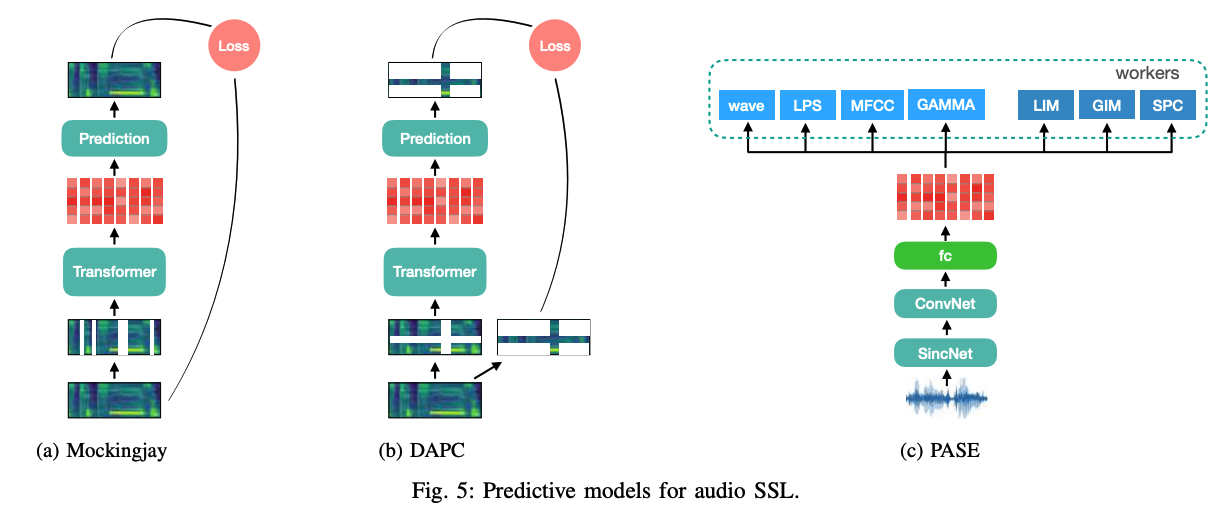
Mockingjay [92]
- takes the Mel-spectrogram as input acoustic features
- exploits transformers to code randomly masked frames into audio representations.
Audio ALBERT [94]
- same network architecture as Mockingjay
- but the parameters are shared across all its transformer encoder layers
  
  $\rightarrow$ achieving a faster inference and increasing training speed
TERA [93]
- TERA = Transformer Encoder Representations from Alteration
- extend the masking procedures
  - ex) replacing contiguous segments with randomness
  - ex) masking along the channel axis
  - ex) applying Gaussian noise

Reconstruct ONLY MASKED : [95]

DAPC [95]
- only predict the missing components along the timeand frequency axes of an audio spectrogram
- can be seen as extension of CBoW
- input masked spectrogram : generated using SpecAugment [34]
  - $\therefore$ the missing parts to be predicted are not only temporal frames, but also frequency bins.

Various pretrain tasks:

PASE [96]
- PASE = problem agnostic speech encoder
- combines a CNN encoder with “multiple neural decoders ( =workers )”
  
  ( aim at solving regression or binary discrimination tasks )
- (1) Regression tasks
  - recovering the raw audio waveform, the log power sepctrogram, MFCCs, and prosody.
- (2) Binary discrimination tasks ( contrastive learning )
  - by maximising local and global mutual information similar.
  $\rightarrow$ Each self-supervised task is expected to provide a different view of the speech signal!
- architecture: SincNet [103]
  - to process the raw waveform as the encoder input
  - performs a convolution with a set of parametrised Sinc functions that implement rectangular band-pass filters.
PASE+ [97]
- Pase+ = PASE + (1) + (2) + (3)
  - (1) additional data augmentation techniques
  - (2) more effective workers
- CNN encoder is combined with a Quasi-Recurrent Neural Network (QRNN)
  - for capturing long-term dependencies in sequential data in a more efficient way

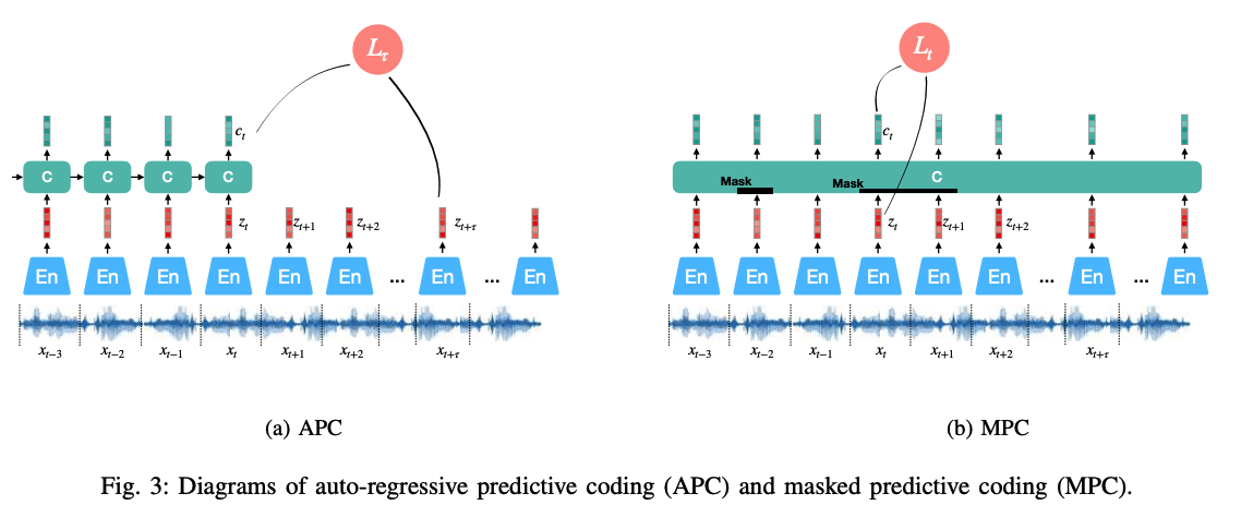
CPC [40]

effectively learn representations by predicting the future in a latent space using an AR model
- promising results for audio, images, text processing, and reinforcement learning.
architecture for Audio …
- (1) “strided CNN” to encode raw audio to its latent representation.
- (2) “GRU-RNN” to aggregate the information from all the past timesteps to form a context vector.
Contrastive learning
- contrast the true future to noise representations, given an aggregated context vector.
- Time-domain data augmentation ( such as WavAugment [98] )
  - ex) pitch modification, additive noise, reverberation, band reject filtering, or time masking

CPC2 [98]

two modifications to CPC
- (1) GRU-RNN of CPC $\rightarrow$ a two-layers LSTM-RNN
- (2) linear prediction network $\rightarrow$ a single multi-head transformer layer

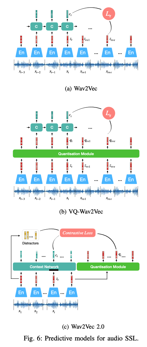
Wav2vec [84]

adjusts the CPC structure to a fully convolutional architecture
- CNN (1) : used to produce a representation from audio
- CNN (2) : captures global context information into a context vector for each time step
substantially improves a character-based ASR system
minimising contrastive loss for each step $k=1, \ldots, K$ :
- $L_k=-\sum_{i=1}^{T-k}\left(\operatorname { l o g } \sigma \left(z_{i+k}^T h_k\left(c_i\right)+\lambda \mathbb{E}\left[\log \sigma\left(-\tilde{z}^T h_k\left(c_i\right)\right]\right)\right.\right.$.
  - \[\sigma(x)=1 /(1+\exp (-x))\]
  - $\sigma\left(z_{i+k}^T h_k\left(c_i\right)\right.$ : the probability of $z_{i+k}$ being the true future sample
  - $h_k\left(c_i\right)=W_k c_i+b_k$.
final loss : $L=\sum_{k=1}^K L_k$

VQ-Wav2vec [85]

similar to a vector-quantised VAE (VQ-VAE)

$\rightarrow$ exploit a vector quantisation module after the wav2vec encoder
aims to find, for each representation, the closest embedding from a fixed size codebook $e \in \mathbb{R}^{V \times d}$
- codebook : contains $V$ representations of size $d$.
“Discrete representations” are fed into the context network & optimised in the same way as for wav2vec.
use Gumbel-Softmax to solve the discontinuity caused by the argmax operation

Mode collapse in single codebook

( Using a single codebook for coding representations tends to mode collapse )

$\rightarrow$ solution : multiple codebooks are used as in product quantisation!

product quantisation = choosing quantised representations from multiple codebooks and concatenating them.
Given $G$ codebooks with $V$ entries $e \in \mathbb{R}^{V x d / G}$, one entry from each codebook is selected.
A linear transformation is applied after concatenating the selected codewords.
probabilities for choosing the $v$-th codebook entry for group $g$ : $p_{g, v}=\frac{e^{\left(l_{g, v}+n_v\right) / \tau}}{\sum_{k=1}^V e^{\left(l_{g, k}+n_k\right) / \tau}}$.
- where $l \in \mathbb{R}^{G \times V}$ represent the logits from projecting the encoded dense representation
- \[n=-\log (-\log (u))\]
  - $u$ are uniform samples from $U(0,1)$
$\rightarrow$ codeword $i$ in group $g$ is chosen by $\operatorname{argmax}_i p_{g, i}$.

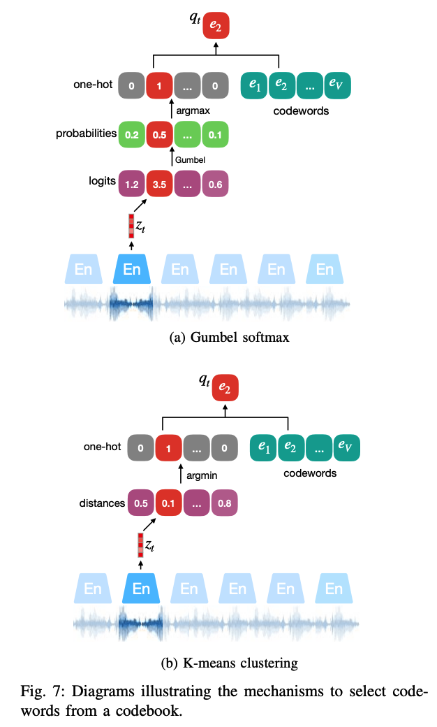
K-means clustering

( = can also be used for differentiable vector quantisation, along with Gumbel Softmax )

codeword is selected as long as it has the closest distance to the dense representations $z$.
additional terms are added in the wav2vec objective function
- $L=\sum_k L_k+\left( \mid \mid \operatorname{sg}(z)-q \mid \mid ^2+\gamma \mid \mid z-\operatorname{sg}(q) \mid \mid ^2\right)$.
term $\mid \mid \operatorname{sg}(z)-q \mid \mid ^2$ = freezes the encoder output $z$ and forces the codewords $Q$ to be closer to the encoder output.
term $\mid \mid z-\operatorname{sg}(q) \mid \mid ^2$ = drives each encoder output to be close to one codeword, which is one centroid of the K-means clustering.

Wave2vec 2.0

Wav2 Vec and VQ-Wav2 Vec : motivated by CPC
- processing audio input for only one forward direction
Wav2vec 2.0
- exploits a bidirectional MPC model
representations ($z$) are partly “MASKED before sending to a transformer network
jointly trained to contrast the true representations from distractors, given the contextualised representations.
similar to VQ-Wav2Vec, Wav2vec 2.0 applies product quantisation to
however, the quantised vector $q_t$ for each time step in Wave2Vec 2.0 is not fed into a context network, but only used in the objective function:
- $L=\mathbb{E}\left[-\log \frac{e^{c_t^T q_t / \tau}}{\sum_{\tilde{q} \sim Q_t} e^{c_t^T \tilde{q} / \tau}}\right]$.
- where $\tilde{q} \sim Q_t$ includes $q_t$ and $K$ distractors.
Regularised by a diversity loss $L_d$
- to encourage the model to use $V$ codebook entries equally often
- $L_d=\frac{1}{G V} \sum_{g=1}^G-H\left(\bar{p}_g\right)=\frac{1}{G V} \sum_{g=1}^G \sum_{v=1}^V \bar{p}_{g, v} \log \bar{p}_{g, v}$.
Wave2vec 2.0 has been explored from the perspective of domain shift in [111]
Findings (1): matching conditions between data of pre-training and testing are very important in order to achieve satisfying speech recognition results.
Findings (2): pre-training on multiple domains can improve the generalisation ability of the learnt representations.

Summary: Wav2vec audio SSL models

learn latent representations without considering specific tasks for pre-training.
After pre-training, they are fine-tuned for downstream tasks in an additional step.
Wav2vec-U [116]
- Wav2vec-U = Wav2vec Unsupervised
- learns a map from audio representations to phonemes directly without supervision.
- GAN architecture
  - $G$: generator uses Wav2vec 2.0 to extract speech representations and generate phoneme sequence based on it using a clustering method
  - $D$ : generated phoneme tries to cheat a $D$ that is conditioned on a real phoneme sequence from unlabelled text.

Phonetic clustering in SeqRAAE [87]

The idea of grouping quantised audio representations into phoneme sequences
discrete representation is learnt in an AE architecture with vector quantisation.
consecutive repeated quantised representations are further grouped to form phonetic units

( = Each phoneme can therefore correspond to several repeated codewords, which is similar to the format of Connectionist Temporal Classification (CTC) [117] )

Hidden unit BERT (HuBERT) [99]

does not apply CL for training the same MPC model and avoids vector quantisation.
each of the learnt audio representation is paired with a pseudo-label provided by applying K-means to MFCCs of the input audio
benefits from cluster ensembles

( $\because$ K-means clustering can be of different numbers of clustering centres = targets of different granularity )

Methods for speech enhancement (SE) task [118], [119]

share similar structure with the auto-encoding predictive model
goal: noisy audio input $\rightarrow$ clean speech.
- noisy = clean speech + mixed with a noise recording

Very recent works in audio SSL

solve typically challenging tasks, such as
- speech enhancement [120]–[122]
- source separation [123]
CAE (clean auto-encoder) and MAE (mixture auto-encoder) [120]
- a pair of variational auto-encoders
- CAE : encodes clean speech
  - by minimising the reconstruction error of its input spectrogram.
- MAE : encodes a noisy utterance
  - forces the encoded representation into the same latent space of the CAE, by using a cycle-consistency loss terms
- learns a mapping from the domain of mixtures to the domain of clean sounds without using paired training examples.
MixIT [124]
- MixIT = Mixture Invariant Training
- for solving unsupervised sound separation
- Seperation Network
  - Input = a mixture of multiple single-channel acoustic mixtures (MOM)
    - each of the acoustic mixtures is comprised of several speech sources.
  - Goal = decomposes the MOM into separate audio sources
    - then selected to be re-mixed up to approximate each acoustic mixture of the MOM.
  - ( Similarly as for the Permutation Invariant Training (PIT) [125]) the remix matrix is optimised by choosing the best match between the separated sources and the acoustic mixtures )
Denoising pretraining [123]
- alternative solution to solve the permutation switching problem of source separation
- pretraining task = speech denoising
- fine-tuned task = source separation

PSE ( SE system specialised in a particular person )

two SSL algorithms :
- (1) pseudo speech enhancement (PseudoSE)
- (2) Contrastive mixtures (CM)
for extracting speaker-specific discriminative features.
(1) PseudoSE model
- trained to recover a premixture signal from a pseudo-source
  - premixture signal = clean speech contaminated by noise
  - pseudo-source = a mixup of the premixture signal and additional noise
(2) CM method
- generalises the training via contrastive learning
- positive & negative
  - positive : shares the same premixture signal (but deformed with different additional noises),
  - negative : stems from two different premixture sources mixed with the same additional noise.
- trained to recover premixture sources rather than clean speech

Data purification (DP) [126]

introduced in the pseudo speech enhancement training
separate model is trained to estimate the segmental SNR of the premixture signals,

( measuring the different importance of the audio frames )

3. Downstream audio Tasks & Benchmarks

Several different downstream audio tasks have been considered for empirically measuring the audio representation quality!

(1) Automatic Speech Recognition (ASR)
- used for evaluating all Wav2vec based methods [81], [84], [85].
(2) Spekaer Identification [36], [45], [103]
(3) Speech emotion recognition [32], [157]-[159]
(4) Speech machine translation [160]
(5) pitch detection [161]
(6) acoustic scene classification [90]

Will describe some publicly available benchmarks that enable a fair comparisons between different audio SSL algorithms.

(1) Zero resource Speech challenge (ZeroSpeech) [162]

a) Challenge in 2015

task of unsupervised discovery of linguistic units from raw speech in an unknown language
tasks are split into two tracks
- (1) unsupervised sub-word modelling
- (2) spoken term discovery
$\rightarrow$ each focusing on a different level of linguistic structure.

(1) unsupervised sub-word modelling

aims at constructing a representation of speech sounds that is robust to within- and between-speaker variation and supports word identification

(2) spoken term discovery

aims at unsupervised discovery of ‘words’, taking raw speech as input.

b) Challenge in 2017

extend the study for the variants in language and speaker

considering the topic of cross-language generalisation and speaker adaptation

c) Challenge in 2017

to address the problem of a speech synthesiser without any text or phonetic labels.

goal: discover sub-word units in an unsupervised way given raw audio.

d) Challenge in 2021

several tasks for spoken language modelling, based on speech only as well as visually-grounded.

(2) Speech processing Universal PERformance Benchmark (SuperB)

Present a standard and comprehensive testbed for evaluation which can be generally applied to pre-trained models on various tasks.

10 downstream tasks are provided

Phoneme Recognition, Automatic Speech Recognition, Keyword Spotting, Query by Example Spoken Term Detection, Speaker Identification, Automatic Speaker Verification, Speaker Diarisation, Intent Classification, Slot Filling, and Emotion Recognition.

(3) LeBenchmark [164]

another reproducible and multifaceted benchmark for evaluating speech SSL models for the French language.

4 tasks

Speech Recognition (ASR), Spoken Language Understanding (SLU), Speech Translation (AST), and Emotion Recognition (AER).

(4) Libri-Light [165]

benchmark specifically designed for the task of ASR with limited or no supervision

based on spoken English audio collected from open-source audio books of the LibriVox project.

(5) HEAR

HEAR = Holistic Evaluation of Audio Representations

extends a benchmark suite for both speech and non-speech tasks
goal : create an audio representation that is as holistic as the human ear

3 main tasks in HEAR 2021

word classification, pitch detection, and sound event detection

Twitter Facebook LinkedIn

Audio Self-supervised Learning; A Survey

Seunghan Lee