Contrastive Audio-Visual Masked Autoencoder

Contrastive Audio-Visual Masked Autoencoder (ICLR 2023)

https://arxiv.org/pdf/2210.07839.pdf

Contents

1. Abstract
2. Introduction
3. CAV-MAE
   1. Preliminaries
   2. AV-MAE
   3. CAV-MAE
4. Experiments

Abstract

Extend MAE from single modality to audio-visual multi-modalities

Propose the Contrastive Audio-Visual Masked Auto-Encoder (CAV-MAE)

• by combining CL & MM, to learn a joint and coordinated audio-visual representation

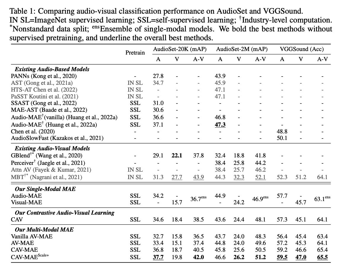
Experiments

• enables the model to perform audio-visual retrieval tasks
• SOTA accuracy of 65.9% on VGGSound

1. Introduction

Acoustic and visual modalities have different properties

Manually annotating audio and video is expensive

• how to utilize web-scale unlabeled video data in a SSL manner has become a core research question.

\(\rightarrow\) Audio-visual self-supervised learning

a) Contrastive Audio-Visual Learning (CAVL)

(Arandjelovic & Zisserman, 2018; Morgado et al., 2021b; Rouditchenko et al., 2021).

• simple yet effective approach

• learns coordinated representations that are closer for paired audio and visual samples than for mismatched samples.
• particularly useful for tasks such as cross-modal retrieval

Limitation : explicitly leverages the very useful audiovisual pair information, but it could discard modality-unique information that is useful in downstram tasks

b) Masked Data Modeling (MDM)

• learns a meaningful representation with the pretext task of recovering the original inputs or features from the corrupted ones (Devlin et al., 2019).
• based on the AST & ViT, the single-modal Masked Auto-Encoder (MAE) (He et al., 2022) achieved state-of-the-art (SOTA) performance on images and audio tasks (Huang et al., 2022a)

Propose to extend the single-modal MAE to Audio-Visual Masked Auto-Encoder (AV-MAE)

• aiming to learn a joint **representation that **fuses the unimodal signals

Limitation : reconstruction task of AV-MAE forces its representation to encode the majority of the input information in the fusion, but it lacks an explicit audio-visual correspondence objective

c) CAV-MAE

Two major SSL frameworks (CAVL & MDM) have been widely used individually,

• they have never been combined in audio-visual learning & they are complementary!

Design the Contrastive Audio-Visual Masked Autoencoder (CAV-MAE)

• integrates CL & MMM
• learns a joint and coordinated audiovisual representation with a single model.

d) Contributions

• (1) extend the single-modal MAE to multi-modal AV-MAE
  • fuses audio-visual inputs for SSL through cross-modal masked data modeling;
• (2) investigate how to best combine CL with MM and propose CAV-MAE
• (3) demonstrate that CL & MM are complementary

2. CAV-MAE

(1) Preliminaries

a) Audio and Image Pre-processing and Tokenization

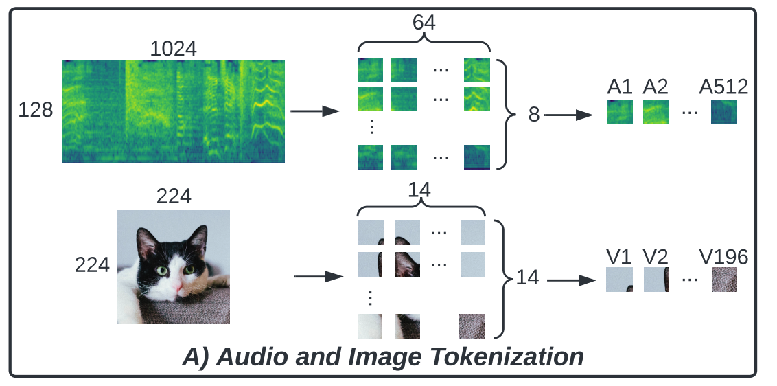
Pre-processing & tokenization

• follow AST (for audio)
• follow ViT (for image)

Dataset

• Pretrain : 10 -second videos (with parallel audios) in AudioSet (Gemmeke et al., 2017)
• Finetune : VGGSound (Chen et al., 2020)

Details ( Audio )

• Step 1) Each 10-second waveform is first converted to a sequence of 128-dimensional log Mel filterbank (fbank) features
  • computed with a \(25 \mathrm{~ms}\) Hanning window every \(10 \mathrm{~ms}\).
  • result : 1024 (time) \(\times 128\) (frequency) spectrogram.
• Step 2) Split the spectrogram into \(51216 \times 16\) square patches \(\mathbf{a}=\left[a^1, \ldots, a^{512}\right]\)

Processing video with Transformer models is expensive

\(\rightarrow\) use frame aggregation strategy

Frame Aggregation Strategy

( concatenating multiple RGB frames : quadratic complexity )

• uniformly sample 10 RGB frames from each 10 -second video (i.e., 1 FPS).

• training & inference

  • training : randomly select one RGB frame as the input
  • inference : average the model prediction of each RGB frame as the video prediction.

• much more efficient with a linear complexity in time

  ( at a cost of not considering inter-frame correlation )

For each RGB frame, we resize and center crop it to \(224 \times 224\), and then split it into \(19616 \times 16\) square patches \(\mathbf{v}=\left[v^1, \ldots, v^{196}\right]\).

b) Transformer Architecture

Each Transformer layer consists of …

• multi-headed self-attention (MSA)
• layer normalization (LN)
• multilayer perceptron (MLP) blocks with residual connections

\(\mathbf{y}=\operatorname{Transformer}(\mathbf{x} ; MSA, LN1, LN2, MLP)\):

• \(\mathbf{y}=\operatorname{MLP}\left(\operatorname{LN}_2\left(\mathbf{x}^{\prime}\right)\right)+\mathbf{x}^{\prime}\).

• \(\mathbf{x}^{\prime}=\operatorname{MSA}\left(\operatorname{LN}_1(\mathbf{x})\right)+\mathbf{x}\).

  • where MSA computes dot-product attention of each element of \(\mathbf{x}\) … quadratic complexity w.r.t. to the size of \(\mathbf{x}\).

c) Contrastive Audio-Visual Learning (CAV)

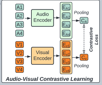
For a mini-batch of \(N\) audio-visual pair samples …

• step1) pre-process and tokenize the audios and images
  • get a sequence of audio and visual tokens \(\left\{\mathbf{a}_i, \mathbf{v}_i\right\}\) for each sample \(i\).
• step 2) input \(\mathbf{a}_i\) and \(\mathbf{v}_i\) to audio and visual Transformer encoders \(\mathrm{E}_{\mathrm{a}}(\cdot)\) and \(\mathrm{E}_{\mathrm{v}}(\cdot)\),
• step 3) get the mean pooled audio and visual representation \(c_i^a\) and \(c_i^v\)
  • \(c_i^a=\operatorname{MeanPool}\left(\mathrm{E}_{\mathrm{a}}\left(\operatorname{Proj}_{\mathrm{a}}\left(\mathbf{a}_i\right)\right)\right.\) and \(c_i^v=\operatorname{MeanPool}\left(\mathrm{E}_{\mathrm{v}}\left(\operatorname{Proj}_{\mathrm{v}}\left(\mathbf{v}_i\right)\right)\right.\),
    • where \(\operatorname{Proj}_{\mathrm{a}}\) and \(\operatorname{Proj}_{\mathrm{v}}\) are linear projections that maps each audio and visual token to \(\mathbb{R}^{768}\).
• step 4) apply a contrastive loss (Equation 7) on \(c_i^a\) and \(c_i^v\).

d) Single Modality Masked Autoencoder (MAE)

For an input sample \(\mathbf{x}\) that can be tokenized as \(\mathbf{x}=\left[x^1, x^2, \ldots, x^n\right]\)…

• step 1) masks a portion of the input \(\mathbf{x}_{\text {mask }}\)
• step 2) only inputs the unmasked tokens \(\mathbf{x} \backslash \mathbf{x}_{\text {mask }}\) to a Transformer
• step 3) reconstruct the masked tokens with the goal of minimizing MSE

Advantages of MAE

• (1) directly uses the original input as the prediction target
  • simplifies the training pipeline.
• (2) only inputs unmaksed tokens to the encoder, and combined with a high masking ratio
  • lowers the computational overhead.
• (3) strong performance in single-modal tasks
  • for both audio and visual modalities.

(2) Vanilla Audio-Visual Masked Autoencoder (AV-MAE)

Has never been applied to audio-visual multi-modality learning.

We extend MAE from a single modality to audio-visual multi-modality and build a “vanilla” audio-visual autoencoder (AV-MAE)

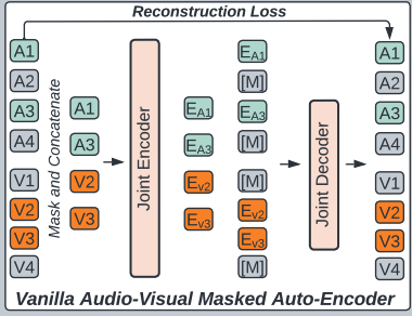
step 1) tokenize a pair of audio and image inputs

• to \(\mathbf{a}=\left[a^1, \ldots, a^{512}\right]\) and \(\mathbf{v}=\left[v^1, \ldots, v^{196}\right]\)

step 2) project them to \(\mathbb{R}^{768}\) with two modal specific linear projection layer

step 3) add a modality type embedding \(\mathbf{E}_{\mathbf{a}}\) and \(\mathbf{E}_{\mathbf{v}}\) & modality specific 2-D sinusoidal positional embedding \(\mathbf{E}_{\mathbf{a}}^{\mathbf{p}}\) and \(\mathbf{E}_{\mathbf{v}}^{\mathbf{p}}\)

• i.e., \(\mathbf{a}^{\prime}=\operatorname{Proj}_{\mathbf{a}}(\mathbf{a})+\mathbf{E}_{\mathbf{a}}+\mathbf{E}_{\mathbf{a}}^{\mathbf{p}}\) and \(\mathbf{v}^{\prime}=\operatorname{Proj}_{\mathbf{v}}(\mathbf{v})+\mathbf{E}_{\mathbf{v}}+\mathbf{E}_{\mathbf{v}}^{\mathbf{p}}\).

step 4) concatenate \(\mathbf{a}^{\prime}\) and \(\mathbf{v}^{\prime}\)

• construct a joint embedding \(\mathbf{x}=\left[\mathbf{a}^{\prime}, \mathbf{v}^{\prime}\right]\).

step 5) mask a portion (75%) of \(\mathbf{x}\)

step 6) only input unmasked tokens \(\mathbf{x}_{\text {unmask }}=\mathbf{x} \backslash \mathbf{x}_{\text {mask }}\) to an audio-visual joint encoder \(\mathrm{E}_{\mathrm{j}}(\cdot)\) and get the output \(\mathrm{x}_{\text {unmask }}^{\prime}\).

step 7) pad \(\mathrm{x}_{\text {unmask }}^{\prime}\) with trainable masked tokens

• at their original position as \(\mathbf{x}^{\prime}\).

step 8) also add modality type embedding \(\mathbf{E}_{\mathbf{a}}^{\prime}\) and \(\mathbf{E}_{\mathbf{v}}^{\prime}\) & modality-specific 2-D sinusoidal positional embedding \(\mathbf{E}_{\mathbf{a}}^{\mathbf{p}^{\prime}}\) and \(\mathbf{E}_{\mathbf{v}} \mathbf{p}^{\prime}\) before feeding \(\mathbf{x}^{\prime}\) to a joint audio-visual decoder \(\mathrm{D}_{\mathrm{j}}(\cdot)\)

step 9) reconstruction

• \(\hat{\mathbf{a}}, \hat{\mathbf{v}}=\mathrm{D}_{\mathrm{j}}\left(\mathbf{x}^{\prime}+\left[\mathbf{E}_{\mathbf{a}}^{\prime}, \mathbf{E}_{\mathbf{v}}^{\prime}\right]+\left[\mathbf{E}_{\mathbf{a}}^{\mathbf{p}^{\prime}}, \mathbf{E}_{\mathbf{v}}^{\mathbf{p}}\right]\right)\) .

• minimize MAE.

Compared with single-modal MAEs, the AV-MAE features a cross-modal masked data modeling objective that allows the model to reconstruct one modality based on the information of another modality, which may help the model learn audio-visual correlation.

Limitations :

• without an explicit objective of encouraging paired audio-visual correspondence, vanilla AV-MAE actually does not effectively leverage the audio-visual pairing information

• using a joint encoder for two modalities allows cross-modal attention, but it also means the two very different modalities are processed with the same weights

  \(\rightarrow\) could lead to a sub-optimal solution.

(3) Contrastive Audo-Visual Masked Autoencoder (CAV-MAE)

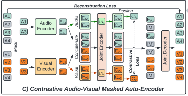
Integrate the complementary advantages of CAV and AVMAE

• design the Contrastive Audio-Visual Masked Autoencoder (CAV-MAE) (shown in Figure 1.C)

For a mini-batch of \(N\) audio-visual pair samples …

• Step 1) pre-process and tokenize the audios and images
  • get a sequence of audio and visual tokens \(\left\{\mathbf{a}_i, \mathbf{v}_i\right\}\) for each sample \(i\)
• step 2) and project them to \(\mathbb{R}^{768}\) with two modal-specific linear projection layer
• step 3) . We also add a modality type embedding \(\mathbf{E}_{\mathbf{a}}\) and \(\mathbf{E}_{\mathbf{v}}\) and modality-specific 2-D sinusoidal positional embedding \(\mathbf{E}_{\mathbf{a}}^{\mathbf{p}}\) and \(\mathbf{E}_{\mathbf{v}}^{\mathbf{p}}\).
• step 4) uniformly mask \(75 \%\) of tokens of each modality
  • \(\mathbf{a}_i^{\text {unmask }} =\operatorname{Mask}_{0.75}\left(\operatorname{Proj}_{\mathrm{a}}\left(\mathbf{a}_i\right)+\mathbf{E}_{\mathbf{a}}+\mathbf{E}_{\mathbf{a}}^{\mathbf{p}}\right)\).
  • \(\mathbf{v}_i^{\text {unmask }} =\operatorname{Mask}_{0.75}\left(\operatorname{Proj}_{\mathbf{v}}\left(\mathbf{v}_i\right)+\mathbf{E}_{\mathbf{v}}+\mathbf{E}_{\mathbf{v}}^{\mathbf{p}}\right)\).

• step 5) input \(\mathbf{a}_i^{\text {unmask }}\) and \(\mathbf{v}_i^{\text {unmask }}\) to independent audio and visual Transformer encoders \(\mathrm{E}_{\mathrm{a}}(\cdot)\) and \(\mathrm{E}_{\mathrm{v}}(\cdot)\) and get \(\mathbf{a}_i^{\prime}\) and \(\mathbf{v}_i^{\prime}\),

• step 6) multi-stream forward passes to input \(\mathbf{a}_i^{\prime}, \mathbf{v}_i^{\prime}\) to a joint audio-visual encoder \(\mathrm{E}_{\mathrm{j}}(\cdot ; \mathrm{MSA}, \mathrm{LN} 1, \mathrm{LN} 2, \mathrm{MLP})\).

  • input 3 things

    • audio tokens \(\mathbf{a}_i^{\prime}\)
    • video tokens \(\mathbf{v}_i^{\prime}\)
    • concatenated audio-visual tokens \(\left[\mathbf{a}_i^{\prime}, \mathbf{v}_i^{\prime}\right]\)

    in three independent forward passes to \(\mathrm{E}_{\mathrm{j}}\).

  • for each stream, we use different layer normalization layers
  • all other weights (i.e., weights of the MSA and MLP) of \(E_j\) are shared for all three streams.
  • \(\begin{array}{r} \left.c_i^a=\operatorname{MeanPool}\left(\mathrm{E}_{\mathrm{j}}\left(\mathrm{E}_{\mathrm{a}}\left(\mathbf{a}_i^{\text {unmask }}\right)\right) ; \mathrm{LN}_{\mathrm{a}}, \mathrm{LN} 2_{\mathrm{a}}\right)\right) \\ \left.c_i^v=\operatorname{MeanPool}\left(\mathrm{E}_{\mathrm{j}}\left(\mathrm{E}_{\mathrm{v}}\left(\mathbf{v}_i^{\text {unmask }}\right)\right) ; \mathrm{LN}_{\mathrm{v}}, \mathrm{LN} 2_{\mathrm{v}}\right)\right) \\ \mathbf{x}_{\mathbf{i}}=\mathrm{E}_{\mathrm{j}}\left(\left[\mathrm{E}_{\mathrm{a}}\left(\mathbf{a}_i^{\text {unmask }}\right), \mathrm{E}_{\mathrm{v}}\left(\mathbf{v}_i^{\text {unmask }}\right)\right] ; \mathrm{LN1}_{\mathrm{av}}, \mathrm{LN}_{\text {av }}\right) \end{array}\).
• step 7) perform 2 tasks
  • (1) CL : with audio and visual single modality stream \(c_i^a\) and \(c_i^v\)
  • (2) MM : with audio-visual multi-modal stream \(\mathbf{x}_{\mathbf{i}}\)

CL

\(\mathcal{L}_{\mathrm{c}}=-\frac{1}{N} \sum_{i=1}^N \log \left[\frac{\exp \left(s_{i, i} / \tau\right)}{\sum_{k \neq i} \exp \left(s_{i, k} / \tau\right)+\exp \left(s_{i, i} / \tau\right)}\right]\).

• where \(s_{i, j}=\mid \mid c_i^v \mid \mid ^T \mid \mid c_j^a \mid \mid\) and \(\tau\) is the temperature.

MM

• pad \(\mathbf{x}_{\mathbf{i}}\) with trainable masked tokens at their original position as \(\mathbf{x}_{\mathbf{i}}^{\prime}\).

• add modality type embedding \(\mathbf{E}_{\mathbf{a}}^{\prime}\) and \(\mathbf{E}_{\mathbf{v}}^{\prime}\) and modality-specific 2-D sinusoidal positional embedding \(\mathbf{E}_{\mathbf{a}}^{\mathbf{p}^{\prime}}\) and \(\mathbf{E}_{\mathbf{v}}^{\mathbf{p}^{\prime}}\)

• feed to a joint audio-visual decoder \(\mathrm{D}_{\mathrm{j}}(\cdot)\) to reconstruct the input audio and image

  • processes audio and visual tokens with a same set of weights except the last modal-specific projection layer ( it outputs \(\hat{\mathbf{a}}_i\) and \(\hat{\mathbf{v}}_i\). )

• Reconstruction loss \(\mathcal{L}_{\mathrm{r}}\) :

  • \(\hat{\mathbf{a}}_i, \hat{\mathbf{v}}_i=\mathrm{D}_{\mathrm{j}}\left(\mathbf{x}^{\prime}+\left[\mathbf{E}_{\mathbf{a}}^{\prime}, \mathbf{E}_{\mathbf{v}}^{\prime}\right]+\left[\mathbf{E}_{\mathbf{a}}^{\mathbf{p}^{\prime}}, \mathbf{E}_{\mathbf{v}}^{\mathbf{p}^{\prime}}\right]\right)\).

  • $$\mathcal{L}{\mathrm{r}}=\frac{1}{N} \sum{i=1}^N\left[\frac{\sum\left(\hat{\mathbf{a}}_i^{\text {mask }}-\operatorname{norm}\left(\mathbf{a}_i^{\text {mask }}\right)\right)^2}{\left

    \mathbf{a}_i^{\text {mask }}\right

    }+\frac{\sum\left(\hat{\mathbf{v}}_i^{\text {mask }}-\operatorname{norm}\left(\mathbf{v}_i^{\text {mask }}\right)\right)^2}{\left

    \mathbf{v}_i^{\text {mask }}\right

    }\right]$$.

    • where \(N\) is the mini-batch size; \(\mathbf{a}^{\text {mask }}, \mathbf{v}^{\text {mask }}, \hat{\mathbf{a}}^{\text {mask }}, \hat{\mathbf{v}}^{\text {mask }}\) denote the original and predicted masked patches

Final Loss

\(\mathcal{L}_{\mathrm{CAV}-\mathrm{MAE}}=\mathcal{L}_{\mathrm{r}}+\lambda_c \cdot \mathcal{L}_{\mathrm{c}}\).

• finetune 0 abandon the decoder and only keep the encoders

3. Experiments