Variational Bayesian Monte Carlo (NeurIPS 2018)
Abstract
Nowadays model : “Expensive, Black-box likelihoods” \(\rightarrow\) hard for Bayesian Inference, due to impracticality
Thus, propose VBMC (Variational Bayesian Monte Carlo)
- novel sample-efficient inference framework
- (1) Variational Inference + (2) GP-based active-sampling Bayesian quadrature
1. Introduction
with Bayesian Inference : parameter & model uncertainty by computing posetrior distn over params & model evidence
-
MCMC & VI
- posterior : \(p(\boldsymbol{x} \mid \mathcal{D})=\frac{p(\mathcal{D} \mid \boldsymbol{x}) p(\boldsymbol{x})}{p(\mathcal{D})}\).
- evidence : \(p(\mathcal{D})=\int p(\mathcal{D} \mid \boldsymbol{x}) p(\boldsymbol{x}) d \boldsymbol{x}\).
- \(p(\mathcal{D} \mid x)\) : likelihood of model …………….Black-box & expensive function
- \(p(x)\): prior
Introduce VBMC (Variational Bayesian Monte Carlo)
- (1) Variational Inference + (2) GP-based active-sampling Bayesian quadrature
- simultaneous approximation of the posterior & of the model evidence in sample-efficient manner
2. Theoretical Background
2-1. Variational Inference
KL-divergence : \(\mathrm{KL}\left[q_{\phi}(x) \mid \mid p(x \mid \mathcal{D})\right]=\mathbb{E}_{\phi}\left[\log \frac{q_{\phi}(x)}{p(x \mid \mathcal{D})}\right]\)
Log-likelihood : \(\log p(\mathcal{D})=\mathcal{F}\left[q_{\phi}\right]+\operatorname{KL}\left[q_{\phi}(x) \mid \mid p(x \mid \mathcal{D})\right] \\\)
ELBO : \(\mathcal{F}\left[q_{\phi}\right]=\mathbb{E}_{\phi}\left[\log \frac{p(\mathcal{D} \mid x) p(x)}{q_{\phi}(x)}\right]=\mathbb{E}_{\phi}[f(x)]+\mathcal{H}\left[q_{\phi}(x)\right]\)
-
\(q\) : chosen to belong to family ( ex. factorized posterior, or mean-field )
providing closed-form equations for coordinate ascent algorithm
-
\(f(x)\) : expensive black-box function
2-2. Bayesian Quadrature
Also known as Bayesian Monte Carlo
-
means to obtain Bayesian estimates of mean & var of non-analytical integrals
of the form \(\langle f\rangle=\int f(\boldsymbol{x}) \pi(\boldsymbol{x}) d \boldsymbol{x}\)
-
\(f\) : function of interest ( ex. GP )
-
\(\pi\) : known pdf
GP (Gaussian Process)
-
prior distn over unknown functions
-
defined by (1) mean & (2) kernel function
-
common choice : ( Gaussian kernel )
\[\kappa\left(\boldsymbol{x}, \boldsymbol{x}^{\prime}\right)=\sigma_{f}^{2} \mathcal{N}\left(\boldsymbol{x} ; \boldsymbol{x}^{\prime}, \boldsymbol{\Sigma}_{\ell}\right),\]with \(\boldsymbol{\Sigma}_{\ell}=\operatorname{diag}\left[\ell^{(1)^{2}}, \ldots, \ell^{(D)^{2}}\right]\)
conditioned on inputs \(\mathbf{X}=\left\{x_{1}, \ldots, x_{n}\right\}\) , GP posterior will have latent posterior conditional mean & covariance :
- mean ) \(\bar{f}_{\Xi}(\boldsymbol{x}) \equiv \bar{f}(\boldsymbol{x} ; \boldsymbol{\Xi}, \psi)\)
- cov ) \(C_{\Xi}\left(\boldsymbol{x}, \boldsymbol{x}^{\prime}\right) \equiv C\left(\boldsymbol{x}, \boldsymbol{x}^{\prime} ; \boldsymbol{\Xi}, \psi\right)\)
Bayesian Integration
Posterior mean & Variance of \(\int f(x) \pi(x) d x\) :
- mean ) \(\mathbb{E}_{f \mid \Xi}[\langle f\rangle]=\int \bar{f}_{\Xi}(x) \pi(x) d x\)
- variance ) \(\mathbb{V}_{f \mid \Xi}[\langle f\rangle]=\iint C_{\Xi}\left(x, x^{\prime}\right) \pi(x) d x \pi\left(x^{\prime}\right) d x^{\prime}\)
if \(f\) has Gaussian kernel & \(\pi\) : (mixture of) Gaussian \(\rightarrow\) can be calculated analytically
Active sampling
given budget of samples \(n_{\max }\)…
- fixed GP hyperparams \(\psi\) : optimal variance-minimizing design does not depend on \(\mathbf{X}\)
- if \(\psi\) updated online : variance of posterior will depend on the function values & active sampling strategy is desirbale
acquisition function : what to choose next?
- \(x_{\text {next }}=\operatorname{argmax}_{x} a(x)\).
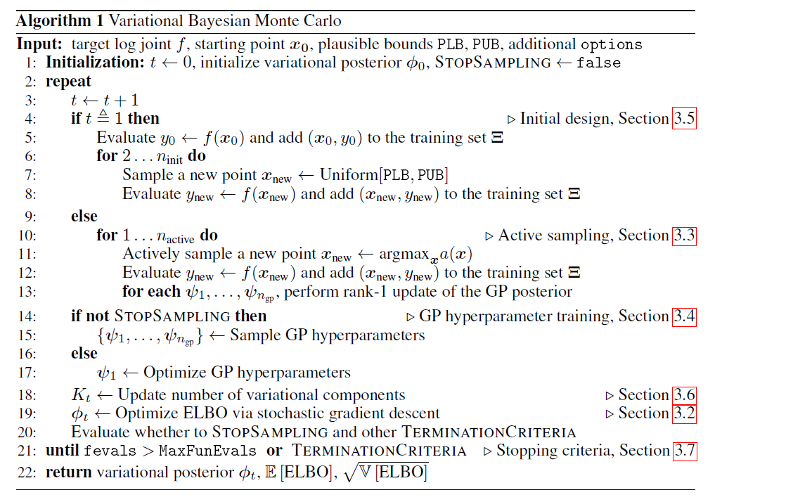
3. Variational Bayesian Monte Carlo ( VBMC )
Simple Algorithm
- 1) sequentially sample
- 2) train GP model
- 3) update variational posterior approximation ( \(\phi_t\) ) by maximizing ELBO
3-1. Variational Posterior
choose variational Posterior \(q(x)\) as “flexible nonparametric” family ( ex. \(K\) Gaussian )
-
\(q(\boldsymbol{x}) \equiv q_{\boldsymbol{\phi}}(\boldsymbol{x})=\sum_{k=1}^{K} w_{k} \mathcal{N}\left(\boldsymbol{x} ; \boldsymbol{\mu}_{k}, \sigma_{k}^{2} \boldsymbol{\Sigma}\right)\).
-
variational posterior : \(\phi \equiv\left(w_{1}, \ldots, w_{K}, \mu_{1}, \ldots, \mu_{K}, \sigma_{1}, \ldots, \sigma_{K}, \lambda\right),\)
( = \(K(D+2)+D\) parameters )
3-2. ELBO
\(\mathcal{F}\left[q_{\phi}\right]=\mathbb{E}_{\phi}\left[\log \frac{p(\mathcal{D} \mid x) p(x)}{q_{\phi}(x)}\right]=\mathbb{E}_{\phi}[f(x)]+\mathcal{H}\left[q_{\phi}(x)\right]\).
[ Approximate ELBO 2 ways ]
(1) approximate log joint probability \(f\)
-
with a GP(Gaussian Process)
-
kernel ) with a Gaussian Kernel
-
mean ) negative quadratic mean function
\(m(\boldsymbol{x})=m_{0}-\frac{1}{2} \sum_{i=1}^{D} \frac{\left(x^{(i)}-x_{\mathrm{m}}^{(i)}\right)^{2}}{\omega^{(i)^{2}}}\).
( unlike constant function, ensures that posterior GP predictive mean \(\bar{f}\) is a proper log prob distn )
-
(2) approximate Entropy \(\mathcal{H}\left[q_{\phi}(x)\right]\)
- via MC sampling ( & propagate using reparam trick )
with (1) & (2), optimize (negative mean) ELBO with SGD!
ELCBO ( Evidence Lower Confidence Bound )
\(\operatorname{ELCBO}(\phi, f)=\mathbb{E}_{f \mid \Xi}\left[\mathbb{E}_{\phi}[f]\right]+\mathcal{H}\left[q_{\phi}\right]-\beta_{\mathrm{LCB}} \sqrt{\mathbb{V}_{f \mid \Xi}\left[\mathbb{E}_{\phi}[f]\right]}\).
- last term : uncertainty in the computation of the expected log joint, multiplied by risk-sensitivity parameter
3-3. Active Sampling
Why? to compute a sequence of integrals \(\mathbb{E}_{\phi_{2}}[f], \ldots, \mathbb{E}_{\phi_{T}}[f]\), such that
- 1) sequence of variational params \(\phi_t\) converges to variational posterior ( that minimizes KL-div )
- 2) have minimum variance on our final estimate of ELBO
2 acquisition functions for VBMC
- 1) Vanilla uncertainty sampling : \(a_{\text {us }}(x)=V_{\Xi}(x) q_{\phi}(x)^{2}\)
- only maximizes the variance under current variational params
- lack exploration
- 2) Prospective uncertainty sampling : \(a_{\mathrm{pro}}(\boldsymbol{x})=V_{\Xi}(\boldsymbol{x}) q_{\phi}(\boldsymbol{x}) \exp \left(\bar{f}_{\Xi}(\boldsymbol{x})\right)\)
- promotes exploration
3-4. Adaptive treatment of GP hyperparameters
GP in VBMC has \(3 D+3\) hyperparams, \(\psi=\left(\ell, \sigma_{f}, \sigma_{\text {obs }}, m_{0}, x_{\mathrm{m}}, \omega\right)\)
-
impose empirical Bayes prior on GP hyperparams, based on current training set
-
sample from the posterior over hyperparams via slice sampling
Given (hyperparam) samples \(\{\psi\} \equiv\left\{\psi_{1}, \ldots, \psi_{n_{\mathrm{gp}}}\right\},\) expected mean & variance :
- mean ) \(\mathbb{E}[\chi \mid\{\psi\}]=\frac{1}{n_{\mathrm{gp}}} \sum_{j=1}^{n_{\mathrm{gp}}} \mathbb{E}\left[\chi \mid \psi_{j}\right]\)
- variance ) \(\mathbb{V}[\chi \mid\{\psi\}]=\frac{1}{n_{\mathrm{gp}}} \sum_{j=1}^{n_{\mathrm{gp}}} \mathbb{V}\left[\chi \mid \psi_{j}\right]+\operatorname{Var}\left[\left\{\mathbb{E}\left[\chi \mid \psi_{j}\right]\right\}_{j=1}^{n_{\mathrm{gp}}}\right]\)
3-5. Initialization and Warm-up
initialized by starting point \(x_0\) & PLB, PUB
- additional points are generated uniformly at random between PLB~PUB ( \(n_{init}=10\) )
Warm-up
-
initialize variational posterior with \(K=2\) components in the vicinity of \(x_0\)
( with small values of \(\sigma_1\), \(\sigma_2\), \(\lambda\) )
-
in warm up mode…
- VBMC quickly improve ELBO by moving to region with higher posterior probability
- collect maximum of \(n_{gp}=8\) hyperparam samples
-
at the end of warm-up….
trim the training set by removing points ( whose log joint prob is more than 10*\(D\) points lower than the max val \(y_{max}\) )
3-6. Adaptive number of variational mixture components
after warm-up… add / remove variational components
ADDING components
- at every iteration, \(K +=1\)
- maximum number of components : \(K_{max} = n^{2/3}\)
REMOVING components
- consider a candidate for pruning \(k\), with mixture weight \(w_k < w_{min}\)
- recompute ELCBO without selected \(k\)