68.Coupled Variational Bayes via Optimization Embedding

Coupled Variational Bayes via Optimization Embedding (NeurIPS 2018)

Abstract

VI’s success depends on two things!

1. Good Approximation
2. Computation Efficiency

Proposes Coupled Variational Bayes, which exploits primal-dual view of ELBO, with variational distribution class generated by optimization embedding

• this flexible function class “couples the variational distribution with original parameters”
• allows end-to-end learning

1. Introduction

Probabilistic models with Bayesian Inference….for

• 1) modeling data with “complex structure”
• 2) “capturing uncertainty”

Choosing proper variational distn is important

• ex) MFVI : reduce computation complexity, but too restricted
• ex) Mixture models & non-parametric family : generalization
  • by introducing more components : more flexible
  • but computational costs increases
• ex) Neural Networks parameterized distributions
• ex) Tractable Flow

using NN for computation tractability restricts expressive ability of the approximation

Not only (1), (2) but also (3) is important!

• (1) approximation error
• (2) computational tractability
• (3) SAMPLE EFFICIENCY

Provides Coupled Variational Bayes (CVB)….2 key components :

• 1) primal-dual view of ELBO
  • avoids computation of determinant of Jacobian ( in flow based model )
• 2) optimization embedding
  • generates an interesting class of variational distn

2. Background

2-1. Variational Inference

ELBO :

• \(\log p_{\theta}(x)=\log \int p_{\theta}(x, z) d z \geqslant \mathbb{E}_{z \sim q_{\phi}(z \mid x)}\left[\log p_{\theta}(x, z)-\log q_{\phi}(z \mid x)\right]\).

Solving above :

• 1) appropriate parameterization for introduced variational distns
• 2) efficient algorithms for updating the params \(\{ \theta, \phi \}\)
  • using SGD

2-2. Reparameterized Density

Recognition model ( Inference Network ) to parameterize variational distribution!

widely used : \(q_{\phi}(z \mid x):=\mathcal{N}\left(z \mid \mu_{\phi_{1}}(x), \operatorname{diag}\left(\sigma_{\phi_{2}}^{2}(x)\right)\right)\)

• where \(\mu_{\phi_{1}}(x)\) and \(\sigma_{\phi_{2}}(x)\) are NN

• such reparams have closed-form of entropy

  \(\rightarrow\) gradient computation & optimization is relatively easy

2-3. Tractable flows-based model

Assume a series of INVERTIBLE transformations as \(\left\{\mathcal{T}_{t}: \mathbb{R}^{r} \rightarrow \mathbb{R}^{r}\right\}_{t=1}^{T}\)

• \(z^{0} \sim q_{0}(z \mid x)\).

  \(z^{T}=\mathcal{T}_{T} \circ \mathcal{T}_{T-1} \circ \ldots \circ \mathcal{T}_{1}\left(z^{0}\right)\).

• \(q_{T}(z \mid x)=q_{0}(z \mid x) \prod_{t=1}^{T}\mid \operatorname{det} \frac{\partial \mathcal{T}_{t}}{\partial z^{t}}\mid^{-1}\).

However, general parameterization of the transformation may violate…

• 1) invertible requirement
• 2) expensive / infeasible calculation for the Jacobian & determinant

3. Coupled Variational Bayes

(1) consider VI from primal-dual view

• avoid computation of determinant of Jacobian

(2) propose the optimization embedding

• generates the variational distribution
• “automatically” produces a non-parametric distribution class ( very flexible )

3-1. A Primal-Dual View of ELBO in Functional Space

Flow based model

• pros) introduce more flexilibity

• cons) calculating determinant of Jacobian introduces extra computational costs

  \(\rightarrow\) with “primal-dual view” , AVOID SUCH COMPUTATION!

ELBO (1) :

\(L(\theta):=\mathbb{E}_{x \sim \mathcal{D}}\left[\log \int p_{\theta}(x, z) d z\right]=\max _{q(z \mid x) \in \mathcal{P}} \underbrace{\mathbb{E}_{x \sim \mathcal{D}} \mathbb{E}_{z \sim q(z \mid x)}\left[\log p_{\theta}(x \mid z)-K L(q(z \mid x) \mid \mid p(z))\right]}_{\ell_{\theta}(q)}\).

• \(p_{\theta}(x, z)=p_{\theta}(x \mid z) p(z)\).

• \(\mathbb{E}_{x \sim \mathcal{D}}[\cdot]\) denotes the expectation over empirical distribution on observations

• \(\ell_{\theta}(q)\) = objective for the variational distrn in density space \(\mathcal{P}\) under the probabilistic model with \(\theta\)

ELBO (2) :

\(L(\theta)=\mathbb{E}_{x \sim \mathcal{D}} \mathbb{E}_{z \sim q_{\hat{\theta}}^{*}(z \mid x)}\left[\log p_{\theta}(x, z)-\log q_{\theta}^{*}(z \mid x)\right]\).

• denote \(q_{\theta}^{*}(z \mid x):=\operatorname{argmax}_{q(z \mid x) \in \mathcal{P}} \ell_{\theta}(q)=\frac{p_{\theta}(x, z)}{\int p_{\theta}(x, z) d z}\)
• can be updated by SGD

• derived, based on Fenchel-duality and interchangeability principle

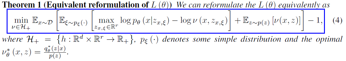
With primal-dual view of ELBO…

• able to represent distribution operation on \(q\), by “local variables \(z_{x,\xi}\)”
  • provides an implicit nonparametric transformation \((x, \xi) \in \mathbb{R}^{d} \times \Xi\) to \(z_{x, \xi} \in \mathbb{R}^{p}\)
  • with the help of dual function \(\nu(x, z)\), can avoid computation of Jacobian

3-2. Optimization Embedding

construct special variational distn, which integrates \(q\)

( i.e transformation on local variables & original parameters of graphical models \(\theta\) )

CANNOT UNDERSTAND….