Normalizing Flows - MAF, IAF, RealNVP

( 참고 : coursera : Probabilistic Deep Learning with Tensorflow2, Tensorflow official website )

Review of Normalizing Flow
Autoregressive Flow
1. Masked Autoregressive Flow (MAF)
2. Inverse Autoregressive Flow (IAF)
Real-NVP & NICE
Training MAF
[ADVANCED] compose multiple bijectors

import numpy as np
import pandas as pd
import matplotlib.pyplot as plt
import tensorflow as tf
import tensorflow_probability as tfp
tfd = tfp.distributions
tfb = tfp.bijectors
tfpl = tfp.layers

1. Review of Normalizing Flow

(1) base distribution :

\(\mathbf{z} \sim N(0, \mathbf{I})\) .

(2) Normalizing Flow :

\(\mathbf{z}_0 = \mathbf{z}\).
\(\mathbf{z}_k = \mathbf{f}_k(\mathbf{z}_{k-1}) \quad k=1, \ldots, K.\).

(3) Log probability :

\(\log p(\mathbf{x}) = \log p(\mathbf{z}) - \sum_{k=1}^K \log \left(\mid \det \left( \frac{\partial \mathbf{f}_k}{\partial \mathbf{z}_{k-1}}(\mathbf{z}_{k-1}) \right) \mid \right)\).
위 식에서, 우리는 determinant of Jacobian을 구해야 한다.

2. Autoregressive Flow

( Autoregressive flow 및 이를 활용한 알고리즘들( MAF, IAF, MADE 등) 에 대한 구체적인 내용은, 이전에 포스트한 논문 리뷰들을 참고하길 바란다. )

핵심은, autoregressive한 형태를 가정하게 될 경우에, Jacobian이 triangular해지고, 따라서 determinant를 쉽게 구할 수 있다 ( by 대각 원소들의 곱으로 )
간단히 수식만 적자면, 아래와 같다.

\(\begin{align} p(x_i \mid\mathbf{x}_{1:i-1}) &= \mathcal{N}(x_i\mid\mu_i, \exp(\sigma_i)^2),\\ \text{where}\qquad \mu_i &= f_{\mu_i}(\mathbf{x}_{1:i-1})\\ \text{and}\qquad \sigma_i &= f_{\sigma_i}(\mathbf{x}_{1:i-1}). \end{align}\).

\(x_i = \mu_i(\mathbf{x}_{1:i-1}) + \exp(\sigma_i(\mathbf{x}_{1:i-1})) z_i \quad \quad i=1, \ldots, D\).

where \(z_i \sim N(0, 1)\)

2-1. Masked Autoregressive Flow (MAF)

\(x\)는 아래와 같은 과정으로 생성(sample)된다.

\(x_1 = f_{\mu_1} + \exp(f_{\sigma_1})z_1\) for \(z_1 \sim N(0, 1)\)
\(x_2 = f_{\mu_2}(x_1) + \exp(f_{\sigma_2}(x_1))z_2\) for \(z_2 \sim N(0, 1)\)
\(x_3 = f_{\mu_3}(x_1, x_2) + \exp(f_{\sigma_3}(x_1, x_2))z_3\) for \(z_3 \sim N(0, 1)\)

여기서 \(f_{\mu_i}\) and \(f_{\sigma_i}\)를 구현하는데에 있어서 MADE(masked autoencoder for distribution estimation)가 사용된다.

weight에 마스킹을 해서 autoregressive한 형태를 만든다
network간의 weight는 서로 공유되어, 총 파라미터수를 줄일 수 있다.

위 식을 바꿔쓰면, 아래와 같이 쓸 수 있다, \(z_i = \frac{x_i - f_{\mu_i}}{\exp(f_{\sigma_i})} \quad \quad i=0, \ldots, D-1\).

이를 통해 알 수 있는 것은, \(z_i\)는 이전의 \(z\)들에 의존하지 않기 떄문에 한번에 (one-pass로) density evaluation을 할 수 있다.

장/단점

장점) \(x\)로부터 “\(z\)를 구하는 것은 빠르다” ( density evaluation은 빠르다 )
단점) \(z\)로부터 “\(x\)를 구하는 것은 느리다” ( sampling은 느리다 )

(1) MADE 네트워크

기본 데이터 및 parameter 설정

params = 2 
event_shape = 3
h = 16

n = 1000
data = tf.random.normal([n,event_shape])

아래와 같이 tfb.AutoregressiveNetwork를 사용하여 MADE를 만든다.

made = tfb.AutoregressiveNetwork(params=params,
                                 event_shape=[event_shape],
                                 hidden_units=[h,h],
                                 activation='sigmoid')

data를 집어넣은 결과 출력되는 output의 size는 다음과 같다.

made(data).shape

TensorShape([1000, 3, 2])

(2) MAF bijector

tfb.MaskedAutoregressiveFlow 함수

MAF_bij = tfb.MaskedAutoregressiveFlow(shift_and_log_scale_fn=MADE)

(3) MAF

tfd.TransformedDistribution 함수

base_normal = tfd.Normal(loc=0,scale=1)
MAF = tfd.TransformedDistribution(base_normal,MAF_bij,event_shape=[event_shape])

2-2. Inverse Autoregressive Flow

Autoregressive Flow의 식 :

\(x_i = \mu_i + \exp(\sigma_i) z_i \quad \quad i=1, \ldots, D\).

하지만, scale/shift function이, \(x_i\)의 함수가 아닌 ’\(z_i\)의 함수’라는 점이 큰 차이점이다.

\(\mu_i = f_{\mu_i}(z_1, \ldots, z_{i-1}) \quad \quad \sigma_i = f_{\sigma_i}(z_1, \ldots, z_{i-1})\).

장/단점

장점) \(z\)로부터 “\(x\)를 구하는 것은 빠르다” ( sampling은 빠르다 )
단점) \(x\)로부터 “\(z\)를 구하는 것은 느리다” ( density evaluation은 느리다 )

(1) MADE 네트워크

앞과 동일

(2) IAF bijector

tfb.Invert & tfb.MaskedAutoregressiveFlow 함수

IAF_bij = tfb.Invert(tfb.MaskedAutoregressiveFlow(shift_and_log_scale_fn=MADE))

(3) IAF

tfd.TransformedDistribution 함수

base_normal = tfd.Normal(loc=0,scale=1)
IAF = tfd.TransformedDistribution(base_normal,IAF_bij,event_shape=[event_shape])

3. Real-NVP & NICE

\(\begin{align} x_i &= z_i \qquad &i = 1, \ldots, d \\ x_i &= \mu_i + \exp(\sigma_i) z_i \qquad &i = d+1, \ldots D \end{align}\).

where \(\mu_i = f_{\mu_i}(z_1, \ldots, z_{d})\) & \(\sigma_i = f_{\sigma_i}(z_1, \ldots, z_{d})\).

앞의 \(d\)차원은 transform X , 뒤에 \(D-d\)차원은 transform O
forward and backward pass 둘 다 parallel하게 처리 가능

( NICE는 Real-NVP에서 scale=1인 version이다 )

(1) NETWORK

tfb.real_nvp_default_template : Build a scale-and-shift function using a multi-layer neural network.

shift_and_log_scale_fn = tfb.real_nvp_default_template(
    hidden_layers=[h,h],activation=tf.nn.relu)

# NICE로 하고 싶으면 ( scale = 1)
shift_and_log_scale_fn = tfb.real_nvp_default_template(
    hidden_layers=[h,h],activation=tf.nn.relu, shift_only=True)

(2) RealNVP_bijector

# (1) masking - 비율로 지정해주기
RealNVP_bij = tfb.RealNVP(
    fraction_masked=0.5,shift_and_log_scale_fn=shift_and_log_scale_fn)
    
# (2) masking - 차원 개수로 지정해주기
d = int(0.5*D)
RealNVP_bij = tfb.RealNVP(
	num_maksed=d,shift_and_log_scale_fn=shift_and_log_scale_fn)

(3) RealNVP

base_mvn = tfd.MultivariateNormalDiag(loc=[0.,0.,0.])
RealNVP = tfd.TransformedDistribution(distribution=base_mvn,bijector=RealNVP_bij)

(4) Combine multiple RealNVP layer

permute = tfp.bijectors.Permute(permutation=[1,2,0])

RealNVP_bij1 = tfb.RealNVP(
    fraction_masked=0.5,shift_and_log_scale_fn=tfb.real_nvp_default_template(hidden_layers=[h,h]))
RealNVP_bij2 = tfb.RealNVP(
    fraction_masked=0.5,shift_and_log_scale_fn=tfb.real_nvp_default_template(hidden_layers=[h,h]))
RealNVP_bij3 = tfb.RealNVP(
    fraction_masked=0.5,shift_and_log_scale_fn=tfb.real_nvp_default_template(hidden_layers=[h,h]))

chained_bijs = tfb.Chain([RealNVP_bij3,permute,RealNVP_bij2,permute,RealNVP_bij1])

mvn = tfd.MultivariateNormalDiag(loc=[0.,0.,0.])
RealNVP = tfd.TransformedDistribution(distribution=mvn,bijector=chained_bijs)

4. Training MAF

사이킷선의 make_moons 데이터셋을 사용해서 위에서 배운 MAF (Masked Autoregressive Flow)에 적용해볼 것이다.

(1) Import Dataset

from sklearn import datasets
from sklearn.preprocessing import StandardScaler
n_samples = 1000
noisy_moons = datasets.make_moons(n_samples=n_samples, noise=.05)
X, y = noisy_moons
X_data = StandardScaler().fit_transform(X)
xlim, ylim = [-2, 2], [-2, 2]

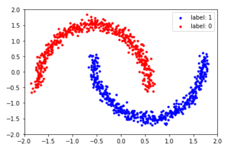
데이터의 모습을 시각화하면 아래와 같다.

y_label = y.astype(np.bool)
X_train, Y_train = X_data[..., 0], X_data[..., 1]
plt.scatter(X_train[y_label], Y_train[y_label], s=10, color='blue')
plt.scatter(X_train[y_label == False], Y_train[y_label == False], s=10, color='red')
plt.legend(['label: 1', 'label: 0'])
plt.xlim(xlim)
plt.ylim(ylim)

(2) MAF 생성

MAF (Masked Autoregressive Flow)를 만들기 위해, 아래의 것들을 생성해야 한다.

1) base distribution
2) MAF bijector
3) trainable distribution

(a) Base distribution

기본 base distribution으로, 평균=0,표준편차=1의 Normal distribution을 잡는다.

base_distn = tfd.Normal(loc=0,scale=1)

(b) MAF bijector

step 1) tfb.AutoregressiveNetwork를 사용하여 MADE (Masked Autoencoder for Distribution Estimation)를 만든다
step 2) tbf.MaskedAutoregressiveFlow의 shift_and_log_scale_fn의 값으로 step1)에서 생성한 MADE를 넣는다.

def make_MAF(hidden_units=[16,16],activation='relu'):
    MADE = tfb.AutoregressiveNetwork(
        params=2,event_shape=[2],
        hidden_units=hidden_units,activation=activation)
    return tfb.MaskedAutoregressiveFlow(shift_and_log_scale_fn=MADE)

(c) Trainable distribution

tfd.TransformedDistribution을 사용하여, base distribution에 bijector를 적용하여 생성한다.

trainable_dist = tfd.TransformedDistribution(base_distn,make_MAF(),
                                            event_shape=[2])

(3) Functions for Visualization

plot_contour_prob : (여러 개의) distribution의 contour plot을 Grid 형식으로 그리는 함수이다.

dist : 그리고자하는 분포들 ( list 형태 )
rows : 시각화할 Grid의 row 개수

def plot_contour_prob(dist, rows=1, title=[''], scale_fig=4):
    cols = int(len(dist) / rows)
    xx = np.linspace(-5.0, 5.0, 100)
    yy = np.linspace(-5.0, 5.0, 100)
    X, Y = np.meshgrid(xx, yy)

    fig, ax = plt.subplots(rows, cols, figsize=(scale_fig * cols, scale_fig * rows))
    fig.tight_layout(pad=4.5)

    i = 0
    for r in range(rows):
        for c in range(cols):
            Z = dist[i].prob(np.dstack((X, Y)))
            if len(dist) == 1:
                axi = ax
            elif rows == 1:
                axi = ax[c]
            else:
                axi = ax[r, c]

            # Plot contour
            p = axi.contourf(X, Y, Z)

            # Add a colorbar
            divider = make_axes_locatable(axi)
            cax = divider.append_axes("right", size="5%", pad=0.1)
            cbar = fig.colorbar(p, cax=cax)

            # Set title and labels
            axi.set_title('Filled Contours Plot: ' + str(title[i]))
            axi.set_xlabel('x')
            axi.set_ylabel('y')
            i += 1
    plt.show()

_plot : 샘플들의 산점도를 그리는 함수이다

def _plot(results, rows=1, legend=False):
    cols = int(len(results) / rows)
    f, arr = plt.subplots(rows, cols, figsize=(4 * cols, 4 * rows))
    i = 0
    for r in range(rows):
        for c in range(cols):
            res = results[i]
            X, Y = res[..., 0].numpy(), res[..., 1].numpy()
            if rows == 1:
                p = arr[c]
            else:
                p = arr[r, c]
            p.scatter(X, Y, s=10, color='red')
            p.set_xlim([-5, 5])
            p.set_ylim([-5, 5])
            p.set_title(names[i])
            
            i += 1

compare_samples_A_B : samples에 담긴 2개의 sample ( 1.정답 샘플 & 2.예측 샘플 )을 시각적으로 비교해보는 함수이다.

def compare_samples_A_B(samples):
    f, arr = plt.subplots(1, 2, figsize=(15, 6))
    names = ['Data', 'Trainable']
    samples = [tf.constant(X_data), samples[-1]]

    for i in range(2):
        res = samples[i]
        X, Y = res[..., 0].numpy(), res[..., 1].numpy()
        arr[i].scatter(X, Y, s=10, color='red')
        arr[i].set_xlim([-2, 2])
        arr[i].set_ylim([-2, 2])
        arr[i].set_title(names[i])

visualize_training_data(samples)

(4) BEFORE train

base distribution에서 (1000,2) shape의 샘플을 뽑은 뒤, (학습되기 이전의) MAF에 적용하여 어떻게 생겼는지 그려보자.

sampling & pass through bijector

trainable_dist.bijector.forward(x) 를 통해, 원하는 샘플을 bijector에 통과시킬 수 있다.

x = base_distn.sample((1000,2))
names = [base_distn.name,trainable_dist.bijector.name]
samples = [x,trainable_dist.bijector.forward(x)]

Visualization

_plot(samples, names,rows=1, legend=False)

(5) Train

from tensorflow.keras.layers import Input
from tensorflow.keras import Model
from tensorflow.keras.callbacks import LambdaCallback

MAF를 학습하기 위한 train_flow함수는 아래와 같다.

optimizer : Adam optimizer
loss : NLL

def train_flow(trainable_distribution,target_X, n_epochs=200, batch_size=None, n_disp=100):
    ######## (1) Define data shape ########################
    n = target_X.shape[0]
    dim = target_X.shape[1]
    
    ######## (2) Make model ################################
    x_ = Input(shape=(dim,), dtype=tf.float32)
    log_prob_ = trainable_distribution.log_prob(x_)
    model = Model(x_, log_prob_)
    model.compile(optimizer=tf.optimizers.Adam(),
                  loss=lambda _, log_prob: -log_prob)

    if batch_size is None:
        batch_size = n
        
	######## (3) Call back ################################
    epoch_callback = LambdaCallback(
        on_epoch_end=lambda epoch, logs: 
                        print('\n Epoch {}/{}'.format(epoch+1, n_epochs, logs),
                              '\n\t ' + (': {:.4f}, '.join(logs.keys()) + ': {:.4f}').format(*logs.values()))
                                       if epoch % n_disp == 0 else False)

	######## (4) Train model ################################
    history = model.fit(x=target_X, y=np.zeros((n, 0), dtype=np.float32),
                        batch_size=batch_size, epochs=n_epochs,
                        validation_split=0.2,shuffle=True,
                        verbose=False,callbacks=[epoch_callback])
    return history

epoch을 600으로해서 학습시킨 결과는 아래와 같다.

history = train_flow(trainable_dist,X_data,n_epochs=600,n_disp=60)

Epoch 1/600 
	 loss: 2.8013, val_loss: 2.7621

 Epoch 61/600 
	 loss: 2.6654, val_loss: 2.6097

 Epoch 121/600 
	 loss: 2.6282, val_loss: 2.5701

 Epoch 181/600 
	 loss: 2.5682, val_loss: 2.5110

 Epoch 241/600 
	 loss: 2.4571, val_loss: 2.4109

 Epoch 301/600 
	 loss: 2.2855, val_loss: 2.2625

 Epoch 361/600 
	 loss: 2.1901, val_loss: 2.1973

 Epoch 421/600 
	 loss: 2.1479, val_loss: 2.1778

 Epoch 481/600 
	 loss: 2.1173, val_loss: 2.1621

 Epoch 541/600 
	 loss: 2.0901, val_loss: 2.1504

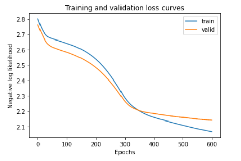
(6) AFTER train

학습 과정에서의 loss가 어떻게 떨어졌는지 확인해보자.

train_losses = history.history['loss']
valid_losses = history.history['val_loss']

plt.plot(train_losses, label='train')
plt.plot(valid_losses, label='valid')
plt.legend()
plt.xlabel("Epochs")
plt.ylabel("Negative log likelihood")
plt.title("Training and validation loss curves")
plt.show()

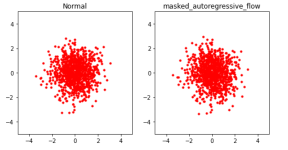
(7) Result & Visualization

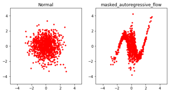
임의로 (1000,2) shape의 샘플을 뽑은 뒤, 이를 (학습이 완료된) 우리의 trainable_dist의 bijector에 forward pass를 해봤다.

x = base_distn.sample((1000,2))
names = [base_distn.name,trainable_dist.bijector.name]
samples = [x,trainable_dist.bijector.forward(x)]

그 결과, make_moons 데이터셋과 유사한 모양을 가짐을 알 수 있다. ( 어느정도 학습이 잘 되어 보인다. )

_plot(samples, names,rows=1, legend=False)

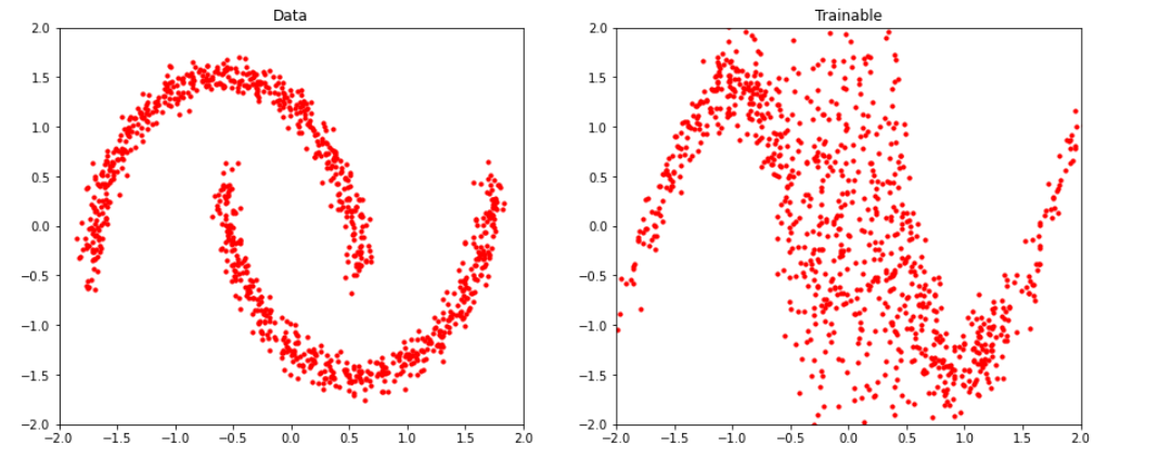
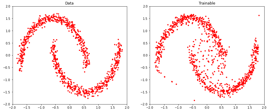
(1) 실제 정답 데이터와, (2) base distn에서 뽑은 뒤 학습시킨 bijector에 통과시킨 우리의 데이터를 비교해보면 아래와 같다.

compare_samples_A_B(samples)

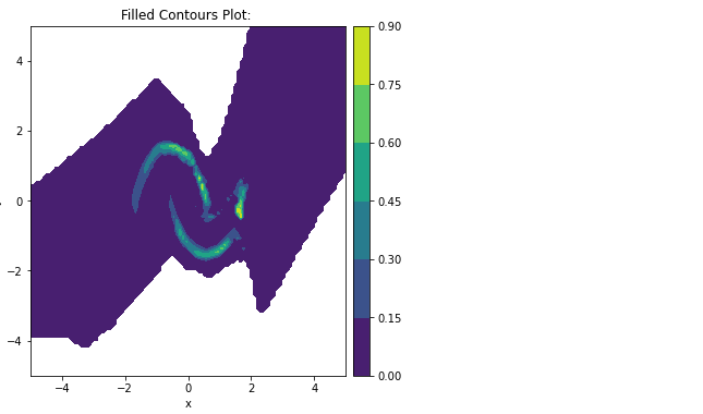
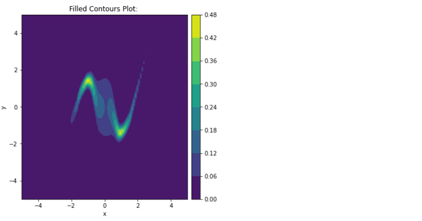
Contour plot을 그려봐도 이와 유사함을 확인할 수 있다.

plot_contour_prob([trainable_dist],scale_fig=6)

5. [ADVANCED] compose multiple bijectors

위의 4.Training MAF에서는 하나의 MAF bijector만을 사용하였다. 하지만 보다 complex한 distribution을 잡아내기 위해선, 더 많은 bijector을 쌓아야 한다. ( compose bijectors! )

tfb.Chain을 사용해서 여러개의 bijector들을 stacking한다.
중간중간에 tfb.Permute을 해줘서, 모든 dimension이 고르게 transform 될 수 있도록 해준다.

num_bijectors=6
bijectors=[]

for i in range(num_bijectors):
    masked_auto_i = make_MAF(hidden_units=[256,256],activation='relu')
    bijectors.append(masked_auto_i)
    bijectors.append(tfb.Permute(permutation=[1,0]))
                     
flow_bijectors = tfb.Chain(list(reversed(bijectors[:-1])))

trainable_dist = tfd.TransformedDistribution(distribution=base_distn,
                                            bijector=flow_bijectors,
                                            event_shape=[2])

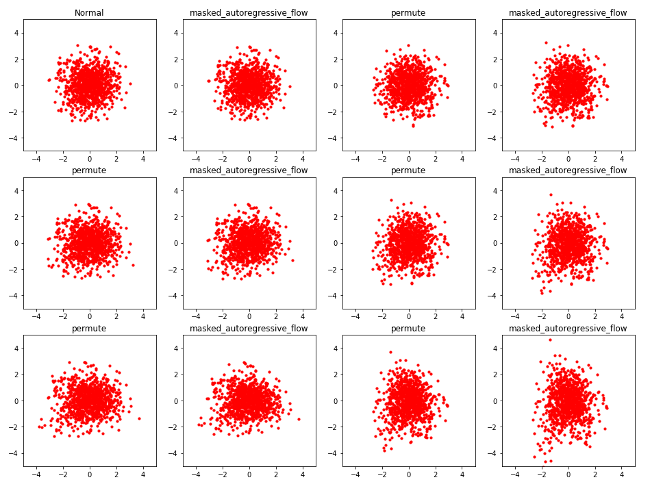
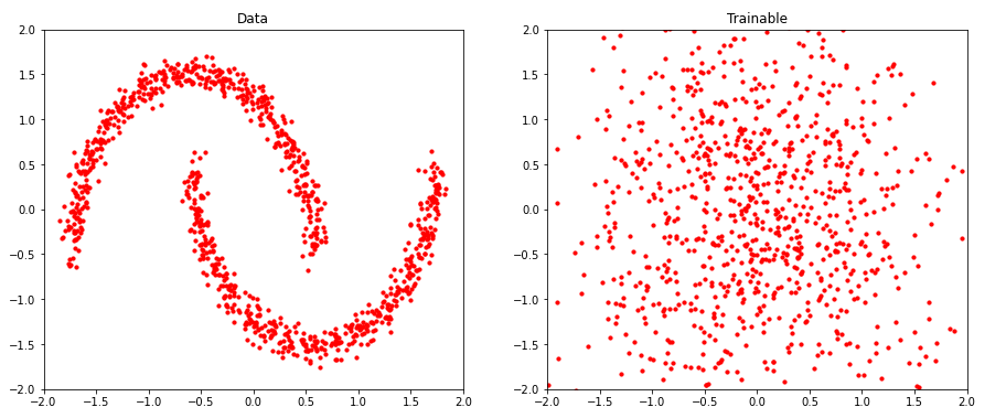
(1000,2)개의 샘플을 만든다. 그리고 이 샘플들이, 각각의 bijector를 통과하면서 그 모습이 어떻게 바뀌는지를 확인해보자.

( base distn에서 처음 뽑힌 sample과, 6개의 bijector와, 그 사이사이에 있는 5개의 permutation까지 총 12개의 sample이 생성한다 )

def make_samples():
    x = base_distn.sample((1000, 2))
    samples = [x]
    names = [base_distn.name]
    for bijector in reversed(trainable_dist.bijector.bijectors):
        x = bijector.forward(x)
        samples.append(x)
        names.append(bijector.name)
    return names, samples
    
names, samples = make_samples()    

아직까지 학습이 이루어지지 않아서, 그 모습이 매우 noisy한 것을 확인할 수 있다.

_plot(samples, names,rows=3, legend=False)

compare_samples_A_B(samples)

이제 학습을 진행해보겠다. Loss가 잘 떨어지고 있는 것을 알 수 있다. 또한, 이전에 bijector를 1개만 사용했을 때보다 성능이 더 좋은 것을 알 수 있다.

history = train_dist_routine(trainable_dist,X_data,n_epochs=600,n_disp=100)

 Epoch 1/600 
	 loss: 2.9205, val_loss: 2.6369

 Epoch 101/600 
	 loss: 2.3190, val_loss: 2.2202

 Epoch 201/600 
	 loss: 2.0324, val_loss: 1.9915

 Epoch 301/600 
	 loss: 2.0080, val_loss: 1.9382

 Epoch 401/600 
	 loss: 1.4850, val_loss: 1.5755

 Epoch 501/600 
	 loss: 1.3063, val_loss: 1.5191

이제 다시 샘플을 뽑은 뒤, 학습이 완료된 MAF에 통과시켜 보겠다. bijector 하나하나를 지날 떄 마다, 그 모습이 어떻게 바뀌는지 확인해보면 아래와 같다.

names, samples = make_samples()
_plot(samples, names,rows=3, legend=False)

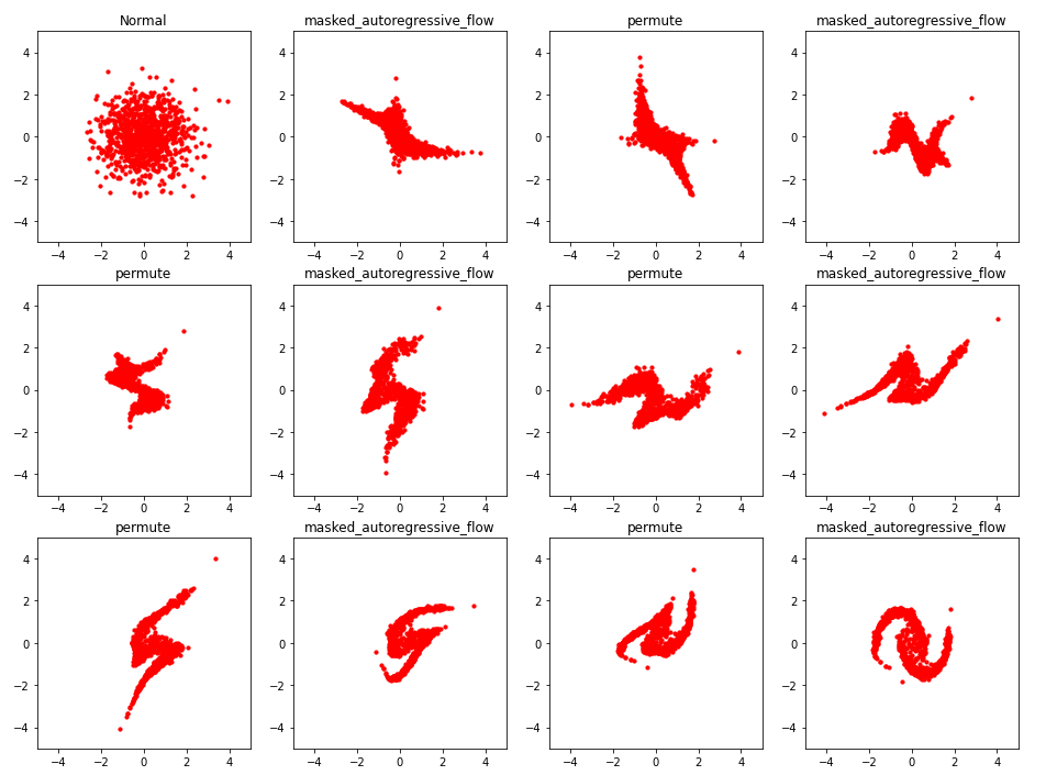
compare_samples_A_B(samples)

plot_contour_prob([trainable_dist],scale_fig=6

Twitter Facebook LinkedIn

(TFP) 11.Normalizing Flows - MAF, IAF, RealNVP

Seunghan Lee

Normalizing Flows - MAF, IAF, RealNVP

Contents

1. Review of Normalizing Flow

2. Autoregressive Flow

2-1. Masked Autoregressive Flow (MAF)

(1) MADE 네트워크

(2) MAF bijector

(3) MAF

2-2. Inverse Autoregressive Flow

(1) MADE 네트워크

(2) IAF bijector

(3) IAF

3. Real-NVP & NICE

(1) NETWORK

(2) RealNVP_bijector

(3) RealNVP

(4) Combine multiple RealNVP layer

4. Training MAF

(1) Import Dataset

(2) MAF 생성

(a) Base distribution

(b) MAF bijector

(c) Trainable distribution

(3) Functions for Visualization

(4) BEFORE train

(5) Train

(6) AFTER train

(7) Result & Visualization

5. [ADVANCED] compose multiple bijectors

You May Also Enjoy