Tensorflow Probability 기본 (1)

( 참고 : coursera : Probabilistic Deep Learning with Tensorflow2, Tensorflow official website )

Distribution
1. Univariate ( Normal, Bernouli )
2. Multivariate
Covariance
1. Full covariance matrix
2. Cholesky Decomposition
Independent
Trainable Distribution

import tensorflow  as tf
import tensorflow_probability as tfp
import matplotlib.pyplot as plt
import seaborn as sns
import numpy as np 
tf.random.set_seed(123)
tfd = tfp.distributions

1. Distribution

1-1. Univariate

(1) Normal Distn

loc : 평균 & scale : 표준편차

normal = tfd.Normal(loc=0.,scale=1.)

normal.sample(5)
normal.sample((3,4)) # or normal.sample([3,4])

normal.prob(0.5)
normal.prob([0.5,0.4])
normal.log_prob(0.5)
normal.log_prob([0.5,0.4])

(2) Bernoulli Distn

bern = tfd.Bernoulli(probs=0.7)
bern2 = tfd.Bernoulli(logits=0.847)

bern : \(p=0.7\)
bern2 : \(\text{log}(\frac{p}{1-p}) = 0.847\)

1-2. Multivariate

쉬운 이해

event shape는 “차원”
batch shape는 “분포의 개수”

(1) Multivariate Normal Distn

mvn = tfd.MultivariateNormalDiag(loc=[-1.,0.5],
                                 scale_diag=[1.,1.5])

batched_normal = tfd.Normal(loc=[-1.,0.5],
                                 scale=[1.,1.5])

mvn : Multivariate 1개 ( : event shape = 2 )
batched_normal = Univariate 2개 ( : batch_shape = 2)

mvn.log_prob([0.1,0.2])
# mvn.log_prob([0.1,0.2,0.3]) -> 에러 ( 2차원에 맞게끔 해야 )

(2) BATCHED Multivariate Normal Distn

batched_mvn = tfd.MultivariateNormalDiag(
    loc=[[-1.,0.5],[2.,0.],[-0.5,1.5]],
    scale_diag=[[1.,1.5],[2.,0.5],[1.,1.]])

batch_shape = 3
event_shape = 2

2. Covariance Matrix

2-1. Full Covariance Matrix

Spherical ( Isotropic ) Gaussian이란?

각 component의 variance가 동일한 경우! & ( random vector being independent )
ex) \(\Sigma = \sigma^2 I\)

Full covariance matrix

Isotropic과는 다르게, correlation이 존재! ( dependent )
tfd.MultivariateNormalTriL를 사용해서 full covariance Gaussian 지정 가능

tfd.MultivariateNormalTriL.

loc : \(\mu\)
scale_tril a lower-triangular matrix \(L\) such that \(LL^T = \Sigma\).

\(d\)-dim r.v에서, lower-triangular matrix \(L\) 는 다음과 같다.

\[\begin{equation} L = \begin{bmatrix} l_{1, 1} & 0 & 0 & \cdots & 0 \\ l_{2, 1} & l_{2, 2} & 0 & \cdots & 0 \\ l_{3, 1} & l_{3, 2} & l_{3, 3} & \cdots & 0 \\ \vdots & \vdots & \vdots & \ddots & \vdots \\ l_{d, 1} & l_{d, 2} & l_{d, 3} & \cdots & l_{d, d} \end{bmatrix}, \end{equation}\]

# (1) Mean
mu = [0., 0.] 

# (2) Covariance
scale_tril = [[1.,  0.],
              [0.6, 0.8]]
sigma = tf.matmul(tf.constant(scale_tril), tf.transpose(tf.constant(scale_tril)))

#-------------------------------------------------
mvn = tfd.MultivariateNormalTriL(loc=mu, scale_tril=scale_tril)

scale_tril에는, \(\Sigma\)가 들어오는 것이 아니라, \(L\)이 들어와야한다

2-2. Cholesky Decomposition

covariance matrix : \(\Sigma = LL^T\). 그렇다면, 왜 \(\Sigma\) 대신 lower-triangular matrix인 \(L\)을 사용해서 표현할까?

Covariance matrix (\(\Sigma\))는 다음의 특성을 따르기 때문이다!

It is symmetric
It is positive (semi-)definite

NB: A symmetric matrix \(M \in \mathbb{R}^{d\times d}\) is positive semi-definite if it satisfies \(b^TMb \ge 0\) for all nonzero \(b\in\mathbb{R}^d\).
If, in addition, we have \(b^TMb = 0 \Rightarrow b=0\) then \(M\) is positive definite.

Cholesky Decomposition는, 위의 특징을 사용하여, symmetric positive-definite matrix \(M\)를 \(LL^T = M\)처럼 분해하는 것을 의미한다. 따라서 우리는 위 2-1에서 말한 것 처럼, covariance matrix를 나타낼 때 tfd.MultivariateNormalTriL.을 사용할 수 있는 것이다.

# (1) Mean
mu = [1., 2., 3.]

# (2) Covariance
sigma = [[0.5, 0.1, 0.1],
         [0.1,  1., 0.6],
         [0.1, 0.6, 2.]]
scale_tril = tf.linalg.cholesky(sigma)

#-------------------------------------------------
mvn = tfd.MultivariateNormalTriL(loc=mu, scale_tril=scale_tril)

3. Independent

tfd.Independent( ,reinterpreted_batch_ndims= )

independent + batch distribution = multivariate distribution ( batch size가 event size로 흡수 됨 )

여러 개의 univariate distn을, (correlation이 서로 0인) multivariate distn으로 묶어줄 수 있다.

# (1) Multivariate distn
mvn = tfd.MultivariateNormalDiag(loc=[-1.,0.5],
                                 scale_diag=[1.,1.5])

# (2) Batch distn
batched_normal = tfd.Normal(loc=[-1.,0.5],
                                 scale=[1.,1.5])

reinterpreted_batch_ndims : controls the number of batch dims which are absorbed as event dims

reinterpreted_batch_ndims=1 : 변환 이후의 event_shape는 [a]

reinterpreted_batch_ndims=2 : 변환 이후의 event_shape는 [a,b]

normal_2d_ind = tfd.Independent(batched_normal,reinterpreted_batch_ndims=1)

결과

batched_normal의 shape : (batch shape=[2], event shape=[])
normal_2d_ind의 shape : (batch shape=[0], event shape=[2])

normal_2d_ind.log_prob([0.2,0.4]))
mvn.log_prob([0.2,0.4])

위의 두 값은 같다. 왜냐하면, mvn의 경우에 서로 correlation이 없는 것으로 지정을 해줬기 때문이다.

4. Trainable Distribution

4-1. Intro & 분포 정의하기

Distribution의 parameter에 constant대신 tf.Variable(xxx)를 넣어주면, 이는 학습가능한 분포로써 정의된다.

Assumption

실제 정답 분포 : rate = 0.3
학습하고자 하는 분포의 initial state : rate = 1.0

# (1) 일반 distn
exponential = tfd.Exponential(rate=0.3,name='exp')

# (2) Trainable Distribution
exp_train = tfd.Exponential(rate=tf.Variable(1.,name='rate'),name='exp_train')
exp_train.trainable_variables

4-2. Loss Function 정의

방금 생성한 Exponential 분포를 학습시켜보겠다.

그러기 위해 우선 loss function을 정의해야하는데, 확률에서 많이 사용하는 nll(negative log likelihood)를 사용하겠다.

def nll(x_train,dist):
    return -tf.reduce_mean(dist.log_prob(x_train))

Loss를 계산하고, 이의 기울기를 구하는 함수 get_loss_and_grad

@tf.function
def get_loss_and_grad(x_train,dist):
    with tf.GradientTape() as tape:
        tape.watch(dist.trainable_variables)
        loss = nll(x_train,dist)
        grads = tape.gradient(loss,dist.trainable_variables)
    return loss,grads

4-3. Train 함수

train_loss에 epoch별로의 train loss를 담는다
train_rates에 epoch별로의 변화하고 있는 parameter ( rate )를 담는다

def exp_dist_optimize(data,dist,n_epoch=15):
    train_loss = []
    train_rate = []
    opt = tf.keras.optimizers.SGD(learning_rate=0.05)
    for epoch in range(1,n_epoch+1):
        loss, grads = get_loss_and_grad(data,dist)
        opt.apply_gradients(zip(grads,dist.trainable_variables))
        rate=dist.rate.value()
        train_loss.append(loss)
        train_rate.append(rate)
        print('Epoch {:03d}:Loss :{:.3f}:Rate:{:.3f}'.format(epoch,loss,rate))
    return train_loss,train_rate

Train data를 임의로 생성한다. (3000개)

아래의 코드를 시행하면, rate=1에서 시작했던 초기값이, 학습이 진행됨에 따라 점차 0.3에 가까워진다.

sampled_data = exponential.sample(3000)
train_loss,train_rate = exp_dist_optimize(data=sampled_data,
                                          dist=exp_train)

Epoch 001:Loss :3.331:Rate:0.883
Epoch 002:Loss :3.067:Rate:0.773
Epoch 003:Loss :2.833:Rate:0.672
Epoch 004:Loss :2.635:Rate:0.579
Epoch 005:Loss :2.476:Rate:0.499
Epoch 006:Loss :2.358:Rate:0.433
Epoch 007:Loss :2.279:Rate:0.382
Epoch 008:Loss :2.235:Rate:0.346
Epoch 009:Loss :2.214:Rate:0.324
Epoch 010:Loss :2.206:Rate:0.312
Epoch 011:Loss :2.204:Rate:0.306
Epoch 012:Loss :2.203:Rate:0.303
Epoch 013:Loss :2.203:Rate:0.301
Epoch 014:Loss :2.203:Rate:0.301
Epoch 015:Loss :2.203:Rate:0.300

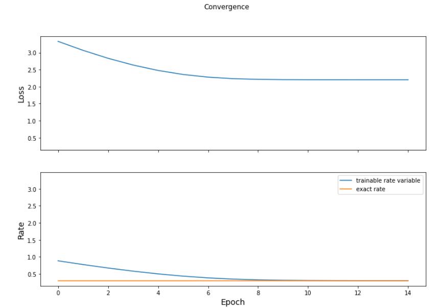
4-4. 결과 비교 및 Visualization

결과 비교

실제 rate : 0.3
예측 rate : 0.3004281

pred_rate = exp_train.rate.numpy()
actual_rate = exponential.rate.numpy()
print(pred_rate,actual_rate)

0.3004281 0.3

exact_value = tf.constant(actual_rate,shape=[len(train_rate)])
fig,axes = plt.subplots(2,sharex=True,sharey=True,figsize=(12,8))
fig.suptitle('Convergence')

axes[0].set_ylabel('Loss',fontsize=14)
axes[0].plot(train_loss)

axes[1].set_xlabel('Epoch',fontsize=14)
axes[1].set_ylabel('Rate',fontsize=14)
axes[1].plot(train_rate,label='trainable rate variable')
axes[1].plot(exact_value,label='exact rate')
axes[1].legend()
plt.show()

Twitter Facebook LinkedIn

(TFP) 07.Tensorflow Probability 기본 (1)

Seunghan Lee