
Tensorflow Probability 기본 (2)
( 참고 : coursera : Probabilistic Deep Learning with Tensorflow2, Tensorflow official website )
Contents
- Distribution Lambda Layer
- Deterministic
- Probabilistic
- Example
- Probabilistic Layer
- Deterministic
- Probabilistic
- Deterministic vs Probabilistic
import tensorflow as tf
import tensorflow_probability as tfp
tfd = tfp.distributions
tfpl = tfp.layers

from tensorflow.keras.models import Sequential
from tensorflow.keras.layers import Dense
from tensorflow.keras.optimizers import RMSprop
from tensorflow.keras.losses import MeanSquaredError
import numpy as np
import matplotlib.pyplot as plt
1. Distribution Lambda Layer
여기서 deterministic / probabilistic의 차이는, output 값이 “fixed” 혹은 “not-fixed”에 있다.
-
Deterministic :
Denselayer만을 사용 -
Probabilistic :
Denselayer와tfpl.DistributionLambda을 함께 사용
1-1. Deterministic
Dense layer만을 사용
Dense의 Input들
- 1) kernel_initializer : WEIGHT의 초기값
- 2) bias_initializer : BIAS의 초기값
model = Sequential([
    Dense(input_shape=(1,), units=1, activation='sigmoid',
          kernel_initializer=tf.constant_initializer(1),
          bias_initializer=tf.constant_initializer(0)),
])
1-2. Probabilistic
tfpl.DistributionLambda(lambda x : tfd.분포(모수=x), convert_to_tensor_fn= )
- step 1) 바로 이전 layer에서 나오게 되는 output값이, 특정
tfd.분포의 모수로 들어가게 된다 - step 2)해당 분포는
convert_to_tensor_fn의 값에 따라, 다른 (최종) output을 낸다.convert_to_tensor_fn=tfd.Distribution.sample: 해당 분포에서 Sample한 값을 출력한다 ( probabilistic )convert_to_tensor_fn=tfd.Distribution.mean: 해당 분포의 Mean을 출력한다 ( deterministic )
model = Sequential([
    Dense(input_shape=(1,), units=1, activation='sigmoid',
          kernel_initializer=tf.constant_initializer(1),
          bias_initializer=tf.constant_initializer(0)),
    tfpl.DistributionLambda(lambda t: tfd.Bernoulli(probs=t),
                           convert_to_tensor_fn=tfd.Distribution.sample)
])
1-3. Example
(a) 가상의 정답 분포 / dataset을 생성
-
weight = 1, bias=0
-
최종 layer :
tfd.Bernoulli( 따라서 activation function으로는 0~1사이 값을 반환하는
activation=sigmoid를 사용한다 )
model = Sequential([
    Dense(input_shape=(1,), units=1, activation='sigmoid',
          kernel_initializer=tf.constant_initializer(1),
          bias_initializer=tf.constant_initializer(0)),
    tfpl.DistributionLambda(lambda t: tfd.Bernoulli(probs=t),
                           convert_to_tensor_fn=tfd.Distribution.sample)
])
x_train = np.linspace(-5, 5, 500)[:, np.newaxis]
y_train = model.predict(x_train)
(b) 학습시킬 분포 생성
-
weight = 2, bias = 2로 임의로 초기값 지정
-
최종 layer :
tfd.Bernoulli( 따라서 activation function으로는 0~1사이 값을 반환하는
activation=sigmoid를 사용한다 )
model_untrained = Sequential([
    Dense(input_shape=(1,), units=1, activation='sigmoid',
          kernel_initializer=tf.constant_initializer(2),
          bias_initializer=tf.constant_initializer(2)),
    tfpl.DistributionLambda(lambda t: tfd.Bernoulli(probs=t),
                           convert_to_tensor_fn=tfd.Distribution.sample)
])
(c) Loss Function 지정
negative log likelihood (nll)
def nll(y_true,y_pred) :
    return -y_pred.log_prob(y_true)
(d) optimizer & model compile
optimizer로 RMSprop ( with learning rate 0.01 )
model_untrained.compile(loss=nll,
                       optimizer=tf.keras.optimizers.RMSprop(learning_rate=0.01))
(e) Train하기
NOT necessary
- epoch별 weight와 bias의 변화를 보기 위한 list를 생성한다
epochs = [0]
training_weights = [model_untrained.weights[0].numpy()[0, 0]]
training_bias = [model_untrained.weights[1].numpy()[0]]
100번의 epoch을 돌면서, 변화하는 weight와 bias를 기록한다.
for epoch in range(100):
    model_untrained.fit(x=x_train, y=y_train, epochs=1, verbose=False)
    epochs.append(epoch)
    training_weights.append(model_untrained.weights[0].numpy()[0, 0])
    training_bias.append(model_untrained.weights[1].numpy()[0])
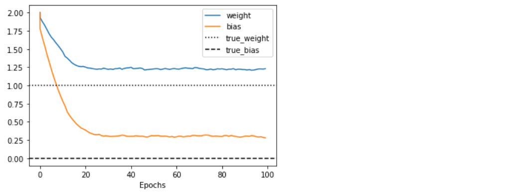
(f) 결과 Visualization
plt.plot(epochs, training_weights, label='weight')
plt.plot(epochs, training_bias, label='bias')
plt.axhline(y=1, label='true_weight', color='k', linestyle=':')
plt.axhline(y=0, label='true_bias', color='k', linestyle='--')
plt.xlabel('Epochs')
plt.legend()
plt.show()
2. Probabilistic Layer
가상 데이터 생성
\(y_i = x_i + \frac{3}{10}\epsilon_i\) where \(\epsilon_i \sim N(0, 1)\) are independent and identically distributed.
x_train = np.linspace(-1, 1, 100)[:, np.newaxis]
y_train = x_train + 0.3*np.random.randn(100)[:, np.newaxis]
Loss Function 생성
- deterministic한 모델은 그냥 RMSE/MSE 등을 쓰면 되지만
- probabilistic한 모델은 아래의
nll( negative log likelihood )를 흔히 사용한다
def nll(y_true,y_pred):
    return -y_pred.log_prob(y_true)
2-1. Deterministic
Denselayer 1개만 이용한다- parameter : 2개 ( weight 1개, bias 1개 )
deter_model = Sequential([
    Dense(units=1, input_shape=(1,))
])
(loss function) MSE
deter_model.compile(loss=MeanSquaredError(), optimizer=RMSprop(learning_rate=0.005))
deter_model.fit(x_train, y_train, epochs=200, verbose=False)
2-2. Probabilistic ( Aleatoric )
Epistemic uncertainty : weight가 uncertain ( deterministic하지 않음))
Aleatoric uncertainty : data 생성과정에서 생기는 uncertainty. \(\rightarrow\) 이번 파트에서는 이것만 다룰 것
tfpl.DistributionLambdalayer를 마지막에 사용한다.- parameter : 2개 ( weight 1개, bias 1개 )
prob_model = Sequential([
    Dense(units=1, input_shape=(1,)),
    tfpl.DistributionLambda(lambda t: tfd.Independent(tfd.Normal(loc=t,scale=1)))
])
- loss function :
nll
prob_model.compile(loss=nll, optimizer=RMSprop(learning_rate=0.005))
prob_model.fit(x_train, y_train, epochs=200, verbose=False)
[TIP] Probabilistic Layer 생성하는 2가지 방법
- 방법 1)
model = Sequential([
    Dense(units=2, input_shape=(1,)),
    tfpl.DistributionLambda(lambda t: tfd.Independent(
        tfd.Normal(loc=t[...,:1],scale=tf.math.softplus(t[...,1:]))))
])
- 방법 2)
event_shape=1

model = Sequential([
    Dense(units=tfpl.IndependentNormal.params_size(event_shape),input_shape=(1,)),
    tfpl.IndependentNormal(event_shape)
])
2-3. Deterministic vs Probabilistic
Output :
- Deterministic : single value
- Probabilsitic : distribution
x = np.array([[0.]])
y_deter_model  = deter_model(x)
y_prob_model  = prob_model(x)
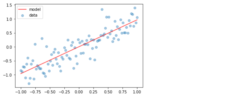
(a) Deterministic 모델 시각화
plt.scatter(x_train, y_train, alpha=0.4, label='data')
plt.plot(x_train, deter_model.predict(x_train), color='red', alpha=0.8, label='model')
plt.legend()
plt.show()
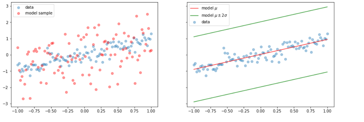
(b) Probabilistic 모델 시각화
y_model = prob_model(x_train)
y_sample = y_model.sample()

y_hat = y_model.mean()
y_sd = y_model.stddev()
y_hat_m2sd = y_hat - 2 * y_sd
y_hat_p2sd = y_hat + 2 * y_sd

fig, (ax1, ax2) = plt.subplots(1, 2, figsize=(15, 5), sharey=True)
ax1.scatter(x_train, y_train, alpha=0.4, label='data')
ax1.scatter(x_train, y_sample, alpha=0.4, color='red', label='model sample')
ax1.legend()
ax2.scatter(x_train, y_train, alpha=0.4, label='data')
ax2.plot(x_train, y_hat, color='red', alpha=0.8, label='model $$\mu$$')
ax2.plot(x_train, y_hat_m2sd, color='green', alpha=0.8, label='model $$\mu \pm 2 \sigma$$')
ax2.plot(x_train, y_hat_p2sd, color='green', alpha=0.8)
ax2.legend()
plt.show()
[ Summary ]
지금까지 위에서 다룬 새로운 probabilistic layer에서 주의해야할 것이 있다. 최종 output값이 분포로 나오고, 따라서 여기서 샘플한 값들은 다르기 때문에 output이 deterministic하지 않다. 하지만, 아직까지 weight는 deterministic하다. 우리는 weight자체에 uncertainty를 부여한 것이 아니라, certain한 weight를, 그냥 그 값 자체가 아닌 특정 분포의 파라미터로써 사용함으로써, 무작위성(uncertainty)가 발생한 것이다. ( 즉, 지금까지 다룬 uncertainty는 aleatoric uncertainty일 뿐이다. )
다음 포스트에서는, weight 자체에 uncertainty를 부여한 모델링을 진행할 것이다. ( with DenseVariationalLayer )