Tensorflow Probability 기본 (3)
( 참고 : coursera : Probabilistic Deep Learning with Tensorflow2, Tensorflow official website )
Contents
- Dense Variational Layer
- Prior & Posterior
- Model
- Result & Visualization
- Epistemic + Aleatoric uncertainty
import tensorflow as tf
import tensorflow_probability as tfp
tfd = tfp.distributions
tfpl = tfp.layers

from tensorflow.keras.models import Sequential
from tensorflow.keras.layers import Dense
from tensorflow.keras.optimizers import RMSprop
from tensorflow.keras.losses import MeanSquaredError
import numpy as np
import matplotlib.pyplot as plt
1. Dense Variational Layer
to capture Epistemic Uncertainty
가상 data 생성
x_train = np.linspace(-1, 1, 100)[:, np.newaxis]
y_train = x_train + 0.3*np.random.randn(100)[:, np.newaxis]
1-1. Prior & Posterior
-
Prior : not trainable, \(MVN(0,I)\)
-
Posterior : trainable, \(MVN(?,?)\)
(a) Prior 정의하기
- input ) weight와 bias의 dimension
- output ) prior model
tfpl.DistributionLambda를 사용하여 “분포” 생성- output = input에서 지정한 차원의 \(MVN(0,I)\)
def prior(kernel_size,bias_size,dtype=None):
    n = kernel_size+bias_size
    prior_model = Sequential([
        tfpl.DistributionLambda(lambda t:tfd.MultivariateNormalDiag(loc=tf.zeros(n),scale_diag=tf.ones(n)))
    ])
    return prior_model
(b) Posterior 정의하기
- input ) weight와 bias의 dimension
- output ) posterior model
- (1)
tfpl.VariableLayer를 사용해서, trainable한 probabilistic layer를 생성한다. - (2) posterior가 따르는 분포
tfpl.MultivariateNormalTriL를 이어서 쌓는다.
- (1)
def posterior(kernel_size,bias_size,dtype=None):
    n = kernel_size+bias_size
    posterior_model = Sequential([
        tfpl.VariableLayer(tfpl.MultivariateNormalTriL.params_size(n),dtype=dtype),
        tfpl.MultivariateNormalTriL(n)
    ])
    return posterior_model
1-2. Model
tfpl.DenseVariational를 사용해서, weight에 uncertainty가 담긴 layer를 만든다.
- 해당 weight는, 앞서 지정한 posterior( + prior )에 따라 그 분포가 결정된다.
다음과 같이 Single-layer NN를 만들 수 있다.
-
make_prior_fn와make_posterior_fn에는, 앞서 만든 prior와 posterior 함수를 넣어 준다. -
kl_weight: (prior와 posterior 사이의) KL-Divergence에 부여하는 weight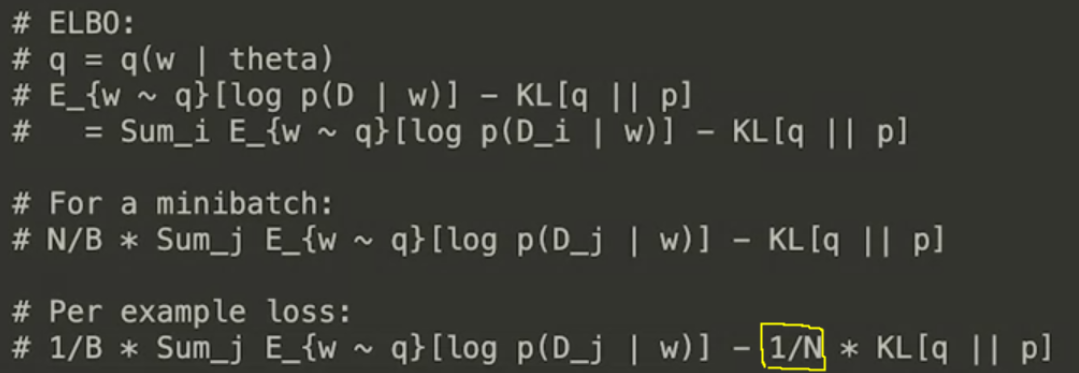
-
kl_use_exact: True일 경우, MC 방법이 아닌 analytical하게 solution을 구한다.
model = Sequential([
    tfpl.DenseVariational(input_shape=(1,),
                         units=1,
                         make_prior_fn=prior,
                         make_posterior_fn=posterior,
                         kl_weight=1/x_train.shape[0],
                         kl_use_exact=True)
])
5개의 parameter가 있는 것을 확인할 수 있다.
model.summary()
- 2개 : MEAN for slope & bias
- 3개 : (CO)VARIANCE
loss : nll이 아니라 MSE이다
- ( \(\because\) 반환되는 값은 single-value이지, distribution이 아님! )
model.compile(loss=MeanSquaredError(),
             optimizer=RMSprop(learning_rate=0.005))
model.fit(x_train,y_train,epochs=500,verbose=False)
1-3. Result & Visualization
아래와 같이 model.layers[i]._prior(), model.layers[i]._posterior()를 통해,
해당 i번째 layer의 prior와 posterior를 불러올 수 있다.
dummy_input = np.array([[103]])
model_prior = model.layers[0]._prior(dummy_input)
model_posterior = model.layers[0]._posterior(dummy_input)

print('prior mean:           ', model_prior.mean().numpy())
print('prior variance:       ', model_prior.variance().numpy())
print('posterior mean:       ', model_posterior.mean().numpy())
print('posterior covariance: ', model_posterior.covariance().numpy()[0])
print('                      ', model_posterior.covariance().numpy()[1])
prior mean:            [0. 0.]
prior variance:        [1. 1.]
posterior mean:        [ 0.93533957 -0.03407374]
posterior covariance:  [0.01383391 0.00173959]
                       [0.00173959 0.00576548]
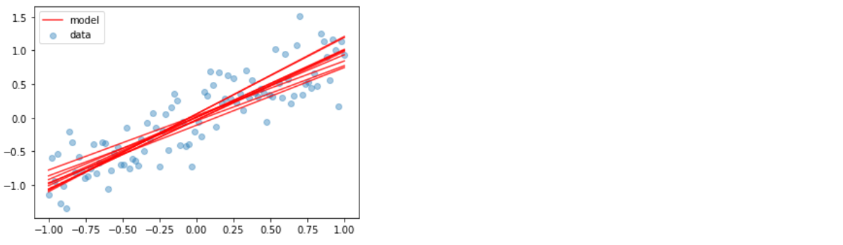
Visualization
plt.scatter(x_train, y_train, alpha=0.4, label='data')
for _ in range(10):
    y_model = model(x_train)
    if _ == 0:
        plt.plot(x_train, y_model, color='red', alpha=0.8, label='model')
    else:
        plt.plot(x_train, y_model, color='red', alpha=0.8)
plt.legend()
plt.show()
2. Epistemic + Aleatoric uncertainty
지난번 포스트의 마지막 부분에서는 “Aleatoric uncertainty”를 반영하는 방법과, 위의 1.에서는 “Epistemic uncertainty”를 반영하기 위한 Dense Variational Layer를 살펴봤다.
이제는, 이 2가지 uncertainty를 모두 모델링한 방법에 대해 알아볼 것이다.
(a) data
x_train = np.linspace(-1, 1, 1000)[:, np.newaxis]
y_train = np.power(x_train, 3) + 0.1*(2+x_train)*np.random.randn(1000)[:, np.newaxis]
(b) model
- prior와 posterior은 1과 동일하게 설정한다.
- 마지막에
tfpl.IndependentNormal(1)를 통해 output값이 분포가 되도록 한다 ( aleatoric uncertainty 반영 )
model = Sequential([
    tfpl.DenseVariational(units=8,
                          input_shape=(1,),
                          make_prior_fn=prior,
                          make_posterior_fn=posterior,
                          kl_weight=1/x_train.shape[0],
                          activation='sigmoid'),
    tfpl.DenseVariational(units=tfpl.IndependentNormal.params_size(1),
                          make_prior_fn=prior,
                          make_posterior_fn=posterior,
                          kl_weight=1/x_train.shape[0]),
    tfpl.IndependentNormal(1)
])
(c) Loss function
- negative log likelihood (
nll)
def nll(y_true, y_pred):
    return -y_pred.log_prob(y_true)
(d) Summary
model.summary()
Model: "sequential_42"
_________________________________________________________________
Layer (type)                 Output Shape              Param #
=================================================================
dense_variational_10 (DenseV (None, 8)                 152
_________________________________________________________________
dense_variational_11 (DenseV (None, 2)                 189
_________________________________________________________________
independent_normal_4 (Indepe ((None, 1), (None, 1))    0
=================================================================
Total params: 341
Trainable params: 341
Non-trainable params: 0
_________________________________________________________________
- (1) 152 개의 parameter
- mean : \(8 \times 2\) = \(16\)
- cov : \(\frac{16^2-16}{2}+16=136\)
- (2) 189개의 parameter
- mean : \((8+1) \times 2\) = \(18\)
- cov : \(\frac{18^2-18}{2}+18=171\)
(e) Train
model.compile(loss=nll, optimizer=RMSprop(learning_rate=0.005))
model.fit(x_train, y_train, epochs=100, verbose=False)
model.evaluate(x_train, y_train)
32/32 [==============================] - 0s 469us/step - loss: 0.2682

0.2682121992111206
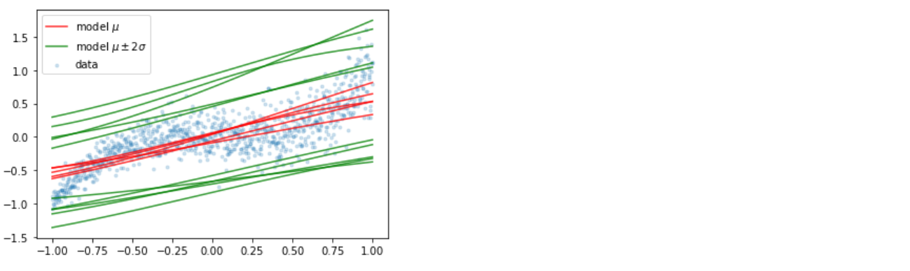
(f) Visualization
-
두 가지 uncertainty 때문에, 똑같은 데이터를 input으로 넣는다고 하더라도 각기 다른 output이 나오게 된다
이를 여러번 반복하여, 어떠한 모델이 피팅되는지 시각화해보자.
plt.scatter(x_train, y_train, marker='.', alpha=0.2, label='data')
for _ in range(5):
    y_model = model(x_train)
    y_hat = y_model.mean()
    y_hat_m2sd = y_hat - 2 * y_model.stddev()
    y_hat_p2sd = y_hat + 2 * y_model.stddev()
    if _ == 0:
        plt.plot(x_train, y_hat, color='red', alpha=0.8, label='model $$\mu$$')
        plt.plot(x_train, y_hat_m2sd, color='green', alpha=0.8, label='model $$\mu \pm 2 \sigma$$')
        plt.plot(x_train, y_hat_p2sd, color='green', alpha=0.8)
    else:
        plt.plot(x_train, y_hat, color='red', alpha=0.8)
        plt.plot(x_train, y_hat_m2sd, color='green', alpha=0.8)
        plt.plot(x_train, y_hat_p2sd, color='green', alpha=0.8)
plt.legend()
plt.show()