(paper 1) SimCLR

A Simple Framework for Contrastive Learning for Visual Representations

Contents

1. Abstract
2. Introduction
3. Method
   1. The Contrastive Learning Framework
   2. Training with Large Batch Size
   3. Evaluation Protocol
4. Data Augmentation for Contrastive Representation Learning

0. Abstract

SimCLR ( = Simple Framework for Contrastive Learning of Visual Representation )

• contrastive SELF-SUPERVISED learning algorithm

  ( without requiring specialized architectures (ex. memory bank) )

3 findings

• (1) composition of data augmentations are important

• (2) introducing a learnable non-linear transformation between “representation” & “contrastive loss” is important

• (3) contrastive learning benefits from..

  • a) larger batch sizes
  • b) more training steps

  than supervised learning

1. Introduction

Generative & Discriminative model

• Generative

  • generate pixels in the input space

  • (cons) pixel-level generation is computationally expensive

    ( + may not be necessary for representation learning )

• Discriminative

  • train NN to perform “pre-text tasks” ( where inputs & labels are from “unlabeled” dataset )
  • (cons) could limit the generality of learned representation

2. Method

(1) The Contrastive Learning Framework

SimCLR learns representations by…

• (1) maximizing agreement between differently augmented versions of same data
• (2) via contrastive loss

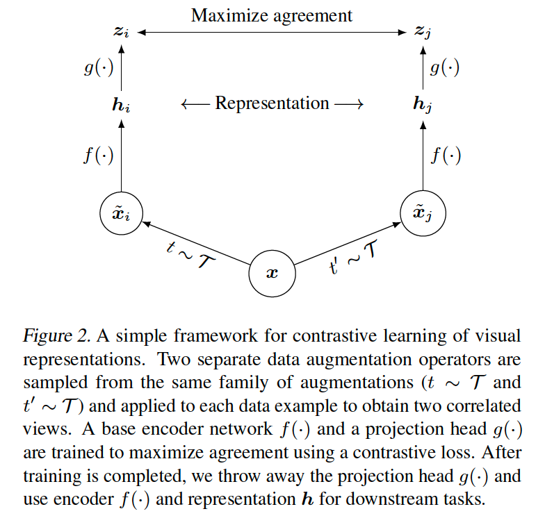
4 major components

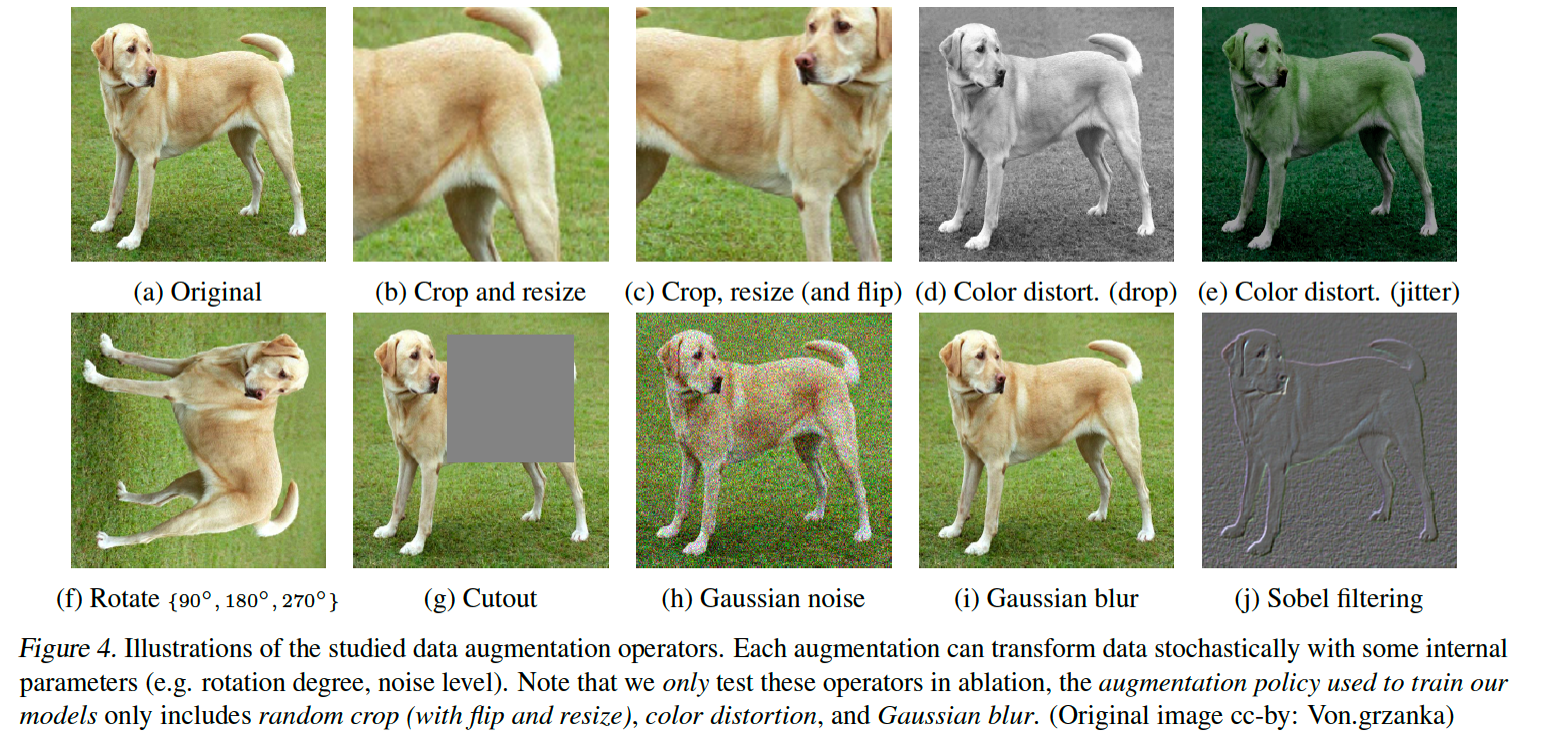
(1) Stochastic data augmentation

• positive pair \(\tilde{x_i}\) & \(\tilde{x_j}\)

• apply 3 simple augmentations

  • (1) random cropping
  • (2) random color distortions
  • (3) random Gaussian blur

  \(\rightarrow\) (1) + (2) : good performance!

(2) Base encoder \(f(\cdot)\)

• \(\boldsymbol{h}_{i}=f\left(\tilde{\boldsymbol{x}}_{i}\right)=\operatorname{ResNet}\left(\tilde{\boldsymbol{x}}_{i}\right)\).
  • where \(\boldsymbol{h}_{i} \in \mathbb{R}^{d}\) is the output after the GAP
  • extract representations from augmented data samples
• use ResNet

(3) Projection head \(g(\cdot)\)

• \(\boldsymbol{z}_{i}=g\left(\boldsymbol{h}_{i}\right)=W^{(2)} \sigma\left(W^{(1)} \boldsymbol{h}_{i}\right)\).
  • maps representations to the space where contrastive loss is applied
• use MLP with 1 hidden layer

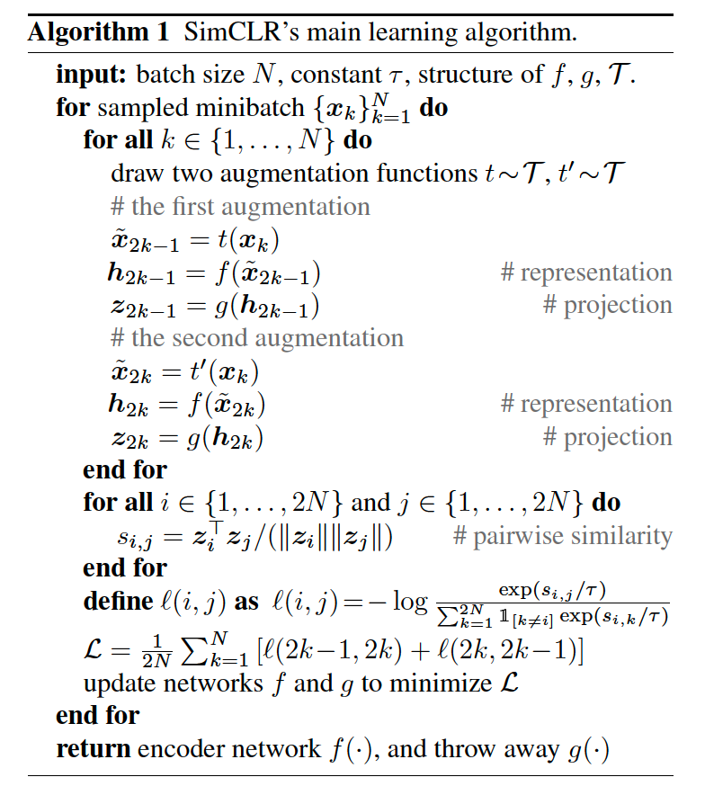
(4) Contrastive loss function

• defined for contrastive prediction task
• Data : set \(\left\{\tilde{\boldsymbol{x}}_{k}\right\}\) including a positive pair ( \(\tilde{\boldsymbol{x}}_{i}\) and \(\tilde{\boldsymbol{x}}_{j}\) )
• Task : aims to identify \(\tilde{\boldsymbol{x}}_{j}\) in \(\left\{\tilde{\boldsymbol{x}}_{k}\right\}_{k \neq i}\) for a given \(\tilde{\boldsymbol{x}}_{i}\).

Sample mini batches of size \(N\)

\(\rightarrow\) 2 augmentations \(\rightarrow\) \(2N\) data points

( no negative samples …only positive pairs )

• Just treat \(2(N-1)\) augmented samples within a mini-batch as negative examples.

Loss Function for a positive pair of examples ( NT-Xent )

( = Normalized Temperature scaled CE loss )

\(\ell_{i, j}=-\log \frac{\exp \left(\operatorname{sim}\left(\boldsymbol{z}_{i}, \boldsymbol{z}_{j}\right) / \tau\right)}{\sum_{k=1}^{2 N} \mathbb{1}_{[k \neq i]} \exp \left(\operatorname{sim}\left(\boldsymbol{z}_{i}, \boldsymbol{z}_{k}\right) / \tau\right)}\).

• where \(\operatorname{sim}(\boldsymbol{u}, \boldsymbol{v})=\boldsymbol{u}^{\top} \boldsymbol{v} / \mid \mid \boldsymbol{u} \mid \mid \mid \mid \boldsymbol{v} \mid \mid\)

\(\rightarrow\) final loss : computed across all positive pairs

(2) Training with Large Batch Size

No memory bank

\(\rightarrow\) instead, vary the training batch size \(N\) from 256 to 8192

( if \(N=8192\) , there are 16382 negative examples per positive pair )

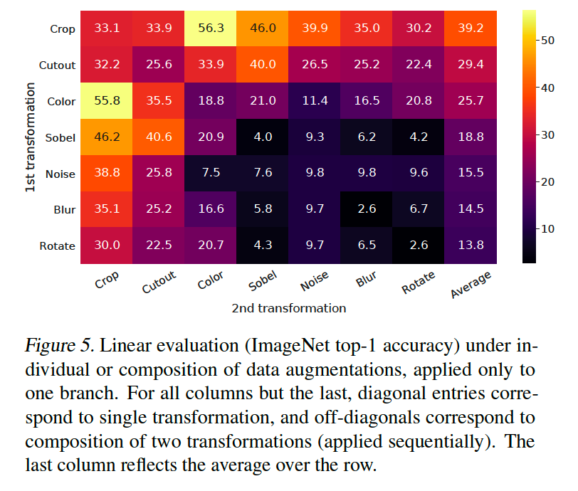
3. Data Augmentation for Contrastive Representation Learning