(paper 18) Contrastive Multiview Coding (CMC)

Contrastive Multiview Coding

Contents

1. Abstract
2. Method
   1. (Review) Predictive Learning methods
   2. Contrastive Learning with 2 views
   3. Contrastive Learning with more than 2 views

0. Abstract

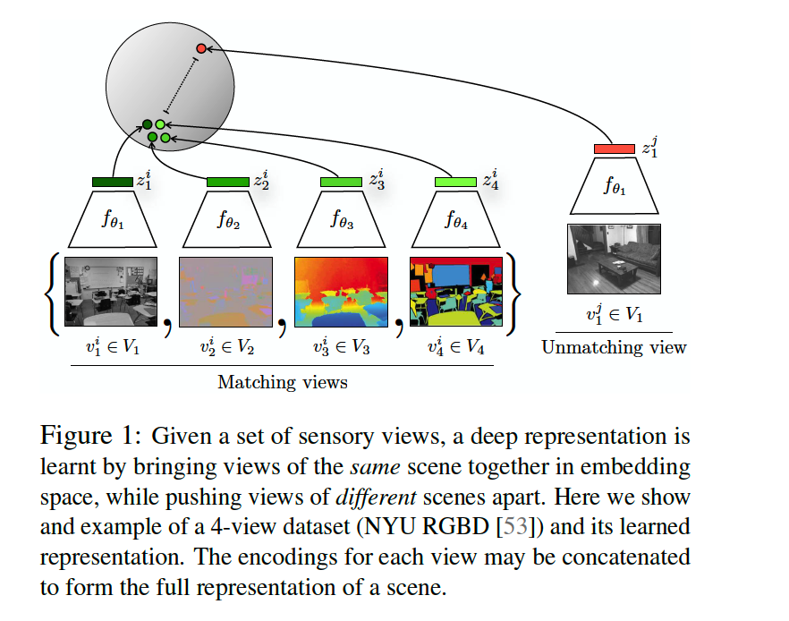
Each view is noisy & incomplete

\(\rightarrow\) but important factors tend to be shared between all vies!

Powerful representation

= representation that models view-invariant factors

\(\rightarrow\) Goal : Learn a representation, that aims to maximize MUTUAL INFORMATION between different views

1. Method

\(V_{1}, \ldots, V_{M}\) : collection of \(M\) views of the data

• \(v_{i} \sim \mathcal{P}\left(V_{i}\right)\).
• ex) \(i=1\) : dark view
• ex) \(i=2\) : bright view

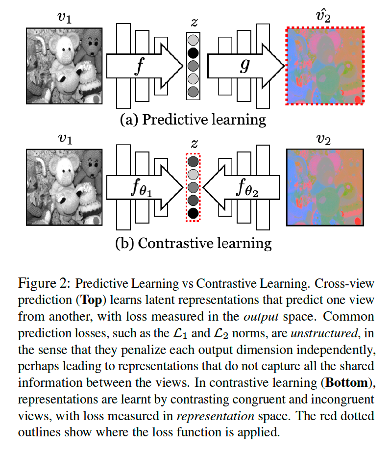
(1) (Review) Predictive Learning methods

Predictive Learning ( = reconstruction based learning )

Notation :

• \(V_{1}\) & \(V_{2}\) : 2 views of a dataset

Predictive Learning setup

• deep non-linear transformation : \(z=f\left(v_{1}\right)\) & \(\hat{v_{2}}=g(z)\)

  • \(f\) : encoder
  • \(g\) : decoder
  • \(\hat{v}_{2}\) : prediction of \(v_{2}\) given \(v_{1}\)

• make \(\hat{v_{2}}\) “close to” \(v_{2}\)

• loss function example : \(\mathcal{L}_{1}\) or \(\mathcal{L}_{2}\) loss function

  \(\rightarrow\) assume independence between each pixel or element of \(v_{2}\) given \(v_{1}\)

  ( = \(p\left(v_{2} \mid v_{1}\right)=\Pi_{i} p\left(v_{2 i} \mid v_{1}\right)\) ….. reduce the ability to model complex structure )

(2) Contrastive Learning with 2 views

Dataset of (\(V_1\) and \(V_2\)) :

• consists of collection of samples \(\left\{v_{1}^{i}, v_{2}^{i}\right\}_{i=1}^{N}\)

  \(\rightarrow\) contrasting congruent and incongruent pairs

• POSITIVE & NEGATIVE

  • POSITIVE ( joint distn ) : \(x=\left\{v_{1}^{i}, v_{2}^{i}\right\}\) , where \(x \sim p\left(v_{1}, v_{2}\right)\)
  • NEGATIVE ( marginal distn ) : \(y=\left\{v_{1}^{i}, v_{2}^{j}\right\}\), where \(y \sim p\left(v_{1}\right) p\left(v_{2}\right)\)

Critic ( = discriminating function ) : \(h_{\theta}(\cdot)\)

\(\rightarrow\) HIGH value for POSITIVE pair, LOW value for NEGATIVE pair

• train to correctly select a single positive sample \(x\) , out of \(S=\left\{x, y_{1}, y_{2}, \ldots, y_{k}\right\}\)
  • 1 positive
  • \(k\) negative

Loss Function :

• \(\mathcal{L}_{\text {contrast }}=-\underset{S}{\mathbb{E}}\left[\log \frac{h_{\theta}(x)}{h_{\theta}(x)+\sum_{i=1}^{k} h_{\theta}\left(y_{i}\right)}\right]\).

• to construct \(S\) …. fix one view & enumerate POS & NEG from other view

  can rewrite it as…

  \(\mathcal{L}_{\text {contrast }}^{V_{1}, V_{2}}=-\underset{\left\{v_{1}^{1}, v_{2}^{1}, \ldots, v_{2}^{k+1}\right\}}{\mathbb{E}}\left[\log \frac{h_{\theta}\left(\left\{v_{1}^{1}, v_{2}^{1}\right\}\right)}{\sum_{j=1}^{k+1} h_{\theta}\left(\left\{v_{1}^{1}, v_{2}^{j}\right\}\right)}\right]\).

  ( view \(V_1\) as anchor & enumrates over \(V_2\) )

a) Implementing the critic

• extract compact latent representations of \(v_1\) & \(v_2\)

  • \(z_{1}=f_{\theta_{1}}\left(v_{1}\right)\).
  • \(z_{2}=f_{\theta_{2}}\left(v_{2}\right)\).

  \(\rightarrow\) compute similarity between \(z_1\) & \(z_2\)

• cosine similarity : \(h_{\theta}\left(\left\{v_{1}, v_{2}\right\}\right)=\exp \left(\frac{f_{\theta_{1}}\left(v_{1}\right) \cdot f_{\theta_{2}}\left(v_{2}\right)}{ \mid \mid f_{\theta_{1}}\left(v_{1}\right) \mid \mid \cdot \mid \mid f_{\theta_{2}}\left(v_{2}\right) \mid \mid } \cdot \frac{1}{\tau}\right)\).

Final loss function : \(\mathcal{L}\left(V_{1}, V_{2}\right)=\mathcal{L}_{\text {contrast }}^{V_{1}, V_{2}}+\mathcal{L}_{\text {contrast }}^{V_{2}, V_{1}}\).

use representation as …

• option 1) \(z_{1}\)
• option 2) \(z_{2}\)
• option 3) \(\left[z_{1}, z_{2}\right]\)

b) Connecting to Mutual Information (MI)

optimal critic \(h_{\theta}^{*}\) : proportional to density ratio between….

• (1) \(p\left(z_{1}, z_{2}\right)\)
• (2) \(p\left(z_{1}\right) p\left(z_{2}\right)\)

\(h_{\theta}^{*}\left(\left\{v_{1}, v_{2}\right\}\right) \propto \frac{p\left(z_{1}, z_{2}\right)}{p\left(z_{1}\right) p\left(z_{2}\right)} \propto \frac{p\left(z_{1} \mid z_{2}\right)}{p\left(z_{1}\right)}\).

\(I\left(z_{i} ; z_{j}\right) \geq \log (k)-\mathcal{L}_{\text {contrast }}\).

• minimizing \(L\) = maximizing the lower bound on MI ( \(I\left(z_{i} ; z_{j}\right))\)
• more negative( \(k\) ) can lead to improved representation

(3) Contrastive Learning with more than 2 views

Generalization of \(\mathcal{L}_{\text {contrast }}^{V_{1}, V_{2}}=-\underset{\left\{v_{1}^{1}, v_{2}^{1}, \ldots, v_{2}^{k+1}\right\}}{\mathbb{E}}\left[\log \frac{h_{\theta}\left(\left\{v_{1}^{1}, v_{2}^{1}\right\}\right)}{\sum_{j=1}^{k+1} h_{\theta}\left(\left\{v_{1}^{1}, v_{2}^{j}\right\}\right)}\right]\).

(1) core view paradigm

(2) full graph paradigm

“core view” paradigm

sets apart one view that we want to optimize over

• ex) if core = \(V_1\) …. build pair-wise representations between \(V_{1}\) and each other view \(V_{j}, j>1\)

by optimizing the sum of a set of pair-wise objectives

• \(\mathcal{L}_{C}=\sum_{j=2}^{M} \mathcal{L}\left(V_{1}, V_{j}\right)\).

“full graph” paradigm

consider all pairs \((i, j), i \neq j\) ( build \(\left(\begin{array}{c}n \\ 2\end{array}\right)\) relationships in all )

objective function :

• \(\mathcal{L}_{F}=\sum_{1 \leq i<j \leq M} \mathcal{L}\left(V_{i}, V_{j}\right)\).