(paper 27) Boosting Few-Shot Visual Learning with Self-Supervision

Boosting Few-Shot Visual Learning with Self-Supervision

Contents

1. Abstract
2. Related Work
   1. Few-shot Learning
   2. Self-supervised Learning
3. Methodology
   1. Explored few-shot learning methods
   2. Boosting few-shot learning via self-supervision

0. Abstract

Few-shot Learning & Self-supervised Learning

• common : how to train a model with little / no-labeled data?

Few-shot Learning :

• how to efficiently learn to recognize patterns in the low data regime

Self-supervised Learning :

• looks into it for the supervisory signal

\(\rightarrow\) this paper exploits both!

1. Related Work

(1) Few-shot Learning

1. Gradient desent-based approach
2. Metric learning based approach
3. Methods learning to map TEST example to a class label by accessing MEMROY modules that store TRAINING examples

This paper : considers 2 approaches from Metric Learning approaches

• (1) Prototypical Network
• (2) Cosine Classifiers

(2) Self-supervised Learning

• annotation-free pretext task
• extracts semantic features that can be useful to other downstream tasks

This paper : considers a mutli-task setting,

• train the bacbone convnet using joint supervision from the supervised end-task
• and an auxiliary self-supervised pretext task

\(\rightarrow\) self-supervision as an auxiliary task will bring improvements

2. Methodology

Few-shot learning : 2 learning stages ( & 2 set of classes )

Notation

• Training set

  • of base classes ( used in 1st stage ) : \(D_b=\{(\mathrm{x}, y)\} \subset I \times Y_b\)
  • of \(N_n\) novel classes ( used in 2nd stage ) : \(D_n=\{(\mathbf{x}, y)\} \subset I \times Y_n\)
    • each class has \(K\) samples ( \(K=1\) or 5 in benchmarks )

  \(\rightarrow\) \(N_n\)-way \(K\)-shot learning

• label sets \(Y_n\) and \(Y_b\) are disjoint

(1) Explored few-shot learning methods

Feature Extractor : \(F_\theta(\cdot)\)

• Prototypical Network (PN), Cosine Classifiers (CC)

  ( difference : CC learns actual base classifiers with feature extractors, while PN simply relies on class-average )

a) Prototypical Network (PN)

[ 1st learning stage ]

• feature extractor \(F_\theta(\cdot)\) is learned on sampled few-shot classification sub-problems

• procedure

  • subset \(Y_* \subset Y_b\) of \(N_*\) base classes ( = support classes ) are sampled

    • ex) cat, dog, ….

  • for each of them, \(K\) training examples are randomly picked from within \(D_b\)

    • ex) (cat1, cat2, .. catK) , (dog1, dog2, … dogK)

    \(\rightarrow\) training dataset \(D_*\)

• prototype : average feature for each class \(j \in Y_*\)

  • \(\mathbf{p}_j=\frac{1}{K} \sum_{\mathbf{x} \in X_*^j} F_\theta(\mathbf{x})\), with \(X_*^j=\left\{\mathbf{x} \mid(\mathbf{x}, y) \in D_*, y=j\right\}\)

• build simple similarity-based classifier with prototype

Output ( for input \(\mathbf{x}_q\) ) :

• for each class \(j\) , the normalized classification score is…

  \(C^j\left(F_\theta\left(\mathbf{x}_q\right) ; D_*\right)=\operatorname{softmax}_j\left[\operatorname{sim}\left(F_\theta\left(\mathbf{x}_q\right), \mathbf{p}_i\right)_{i \in Y_*}\right]\).

Loss function ( of 1st learning stage ) :

• \(L_{\mathrm{few}}\left(\theta ; D_b\right)=\underset{\substack{D_* \sim D_b \\\left(\mathbf{x} q, y_q\right)}}{\mathbb{E}}\left[-\log C^{y_q}\left(F_\theta\left(\mathbf{x}_q\right) ; D_*\right)\right]\).

[ 2nd learning stage ]

• feature extractor is FROZEN
• classifier of novel classes is defined as \(C\left(\cdot ; D_n\right)\)
  • prototypes defined as in \(\mathbf{p}_j=\frac{1}{K} \sum_{\mathbf{x} \in X_*^j} F_\theta(\mathbf{x})\) with \(D_*=D_n\).

b) Cosine Classifiers (CC)

[ 1st learning stage ]

• trains the feature extractor \(F_\theta\) together with a cosine-similarity based classifier
• \(W_b=\left[\mathbf{w}_1, \ldots, \mathbf{w}_{N_b}\right]\) : matrix of the \(d\)-dimensional classification weight vectors
• output : normalized score for image \(x\)
  • \(C^j\left(F_\theta(\mathbf{x}) ; W_b\right)=\operatorname{softmax}_j\left[\gamma \cos \left(F_\theta(\mathbf{x}), \mathbf{w}_i\right)_{i \in Y_b}\right]\).

Loss function ( of 1st learning stage ) :

• \(L_{\mathrm{few}}\left(\theta, W_b ; D_b\right)=\underset{(\mathbf{x}, y) \sim D_b}{\mathbb{E}}\left[-\log C^y\left(F_\theta(\mathbf{x}) ; W_b\right)\right]\).

[ 2nd learning stage ]

• compute one representative feature \(\mathbf{w}_j\) for each new class
  • by averaging \(K\) samples in \(D_n\)
• define final classifier \(C\left(. ;\left[\mathbf{w}_1 \cdots \mathbf{w}_{N_n}\right]\right)\)

(2) Boosting few-shot learning via self-supervision

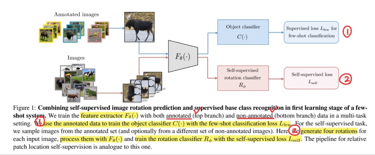
Propose to leverage progress in self-supervised feature learning to improve few-shot learning

[ 1st stage ]

• propose to extend the training of feature extractor \(F_\theta(.)\),

  by including self-supervised task

2 ways to incorporate SSL to few-shot learning

• (1) using an auxiliary loss function, based on self-supervised task
• (2) exploiting unlabeled data in a semi-supervised way

a) Auxiliary loss based on self-supervision

\(\min _{\theta,\left[W_b\right], \phi} L_{\text {few }}\left(\theta,\left[W_b\right] ; D_b\right)+\alpha L_{\mathrm{self}}\left(\theta, \phi ; X_b\right)\).

• by adding auxiliary self-supervised loss in 1st stage

• \(L_{\text {few }}\) : stands for PN few-shot loss / CC loss

Image Rotation

• classes : \(\mathcal{R}=\left\{0^{\circ}, 90^{\circ}, 180^{\circ}, 270^{\circ}\right\}\)
• network \(R_\phi\) predicts the rotation class \(r\)
• \(L_{\text {self }}(\theta, \phi ; X)=\underset{\mathbf{x} \sim X}{\mathbb{E}}\left[\sum_{\forall r \in \mathcal{R}}-\log R_\phi^r\left(F_\theta\left(\mathbf{x}^r\right)\right)\right]\).
  • \(X\) : original training set of non-rotated images
  • \(R_\phi^r(\cdot)\) : predicted normalized score for rotation \(r\)

Relative patch location

• divide it into 9 regions over 3x3 grid

  • \(\overline{\mathrm{x}}^0\) : central image patch
  • \(\overline{\mathrm{x}}^1 \cdots \overline{\mathrm{x}}^8\) : 8 neighbors

• compute the representation of each patch

  & generate patch feature pairs \(\left(F_\theta\left(\overline{\mathbf{x}}^0\right), F_\theta\left(\overline{\mathbf{x}}^p\right)\right)\) by concatenation.

• \(L_{\mathrm{self}}(\theta, \phi ; X)=\underset{\mathbf{x} \sim X}{\mathbb{E}}\left[\sum_{p=1}^8-\log P_\phi^p\left(F_\theta\left(\overline{\mathbf{x}}^0\right), F_\theta\left(\overline{\mathbf{x}}^p\right)\right)\right]\).

  • \(X\) : original training set of non-rotated images
  • \(P_\phi^p\) : predicted normalized score for relative location \(p\).

b) Semi-supervised few-shot learning

• does not depend on class labels
• can obtain information from additional unlabeled data
• \(\min _{\theta,\left[W_b\right], \phi} L_{\mathrm{few}}\left(\theta,\left[W_b\right] ; D_b\right)+\alpha \cdot L_{\mathrm{self}}\left(\theta, \phi ; X_b \cup X_u\right)\).