(paper 28) Self-supervised Label Augmentation via Input Transformations

Self-supervised Label Augmentation via Input Transformations

Contents

1. Abstract
2. Introduction
3. Self-supervised Label Augmentation (SLA)
   1. Multi-task Learning with Self-supervision
   2. Eliminating Invariance via Joint-label Classifier

0. Abstract

self-supervised learning

• constructs artificial labels

This paper :

• constructing artifical labels works well even under fully labeled datasets

• main idea : learn a single unified task w.r.t joint distn of the (1) original labels & (2) self-supervised labels

  ( augment these 2 labels )

• propose a novel knowledge transfser technique ( = self-distillation )

  \(\rightarrow\) faster inference!

1. Introduction

Contribution

1. multi-task approach :

   • enforcing invariance to transformation

     \(\rightarrow\) may lead to bad result in some cases

2. propose a simple & effective algorithm

   • learn a single unified task
   • use joint distribution of original & self-supervised labels

Self-supervised Label Augmentation (SLA)

• proposed label augmentation method

• do not force any invariance to tranfsormation

• assign different labels for each transformation

  \(\rightarrow\) possible to make a prediction by aggregation

  ( act as an ensemble )

• propose a self-distillation technique

  ( transfers knowledge of the multiple inferences into a single inference )

2. Self-supervised Label Augmentation (SLA)

( setting : fully-supervised scenario )

1. problems of conventional multi-task learning approach

2. introduce proposed algorithm

   ( + 2 additional techniques : (1) aggregation & (2) self-distillation )

   • (1) aggregation :

     • uses all differently augmented samples

     • provide an ensemble effect, using a single model

   • (2) self-distillation :

     • transfers the aggregated knowledge into the model itself for acceleration

Notation

• input : \(\boldsymbol{x} \in \mathbb{R}^d\)
• number of classes : \(N\)
• Cross entropy loss : \(\mathcal{L}_{\mathrm{CE}}\)
• softmax classifier : \(\sigma(\cdot ; \boldsymbol{u})\)
  • \(\sigma_i(\boldsymbol{z} ; \boldsymbol{u})=\exp \left(\boldsymbol{u}_i^{\top} \boldsymbol{z}\right) / \sum_k \exp \left(\boldsymbol{u}_k^{\top} \boldsymbol{z}\right)\).
• embedding vector : \(\boldsymbol{z}=f(\boldsymbol{x} ; \boldsymbol{\theta})\)
• augmented sample : \(\tilde{\boldsymbol{x}}=t(\boldsymbol{x})\)
• embedding vector of augmented sample : \(\tilde{\boldsymbol{z}}=f(\tilde{\boldsymbol{x}} ; \boldsymbol{\theta})\)

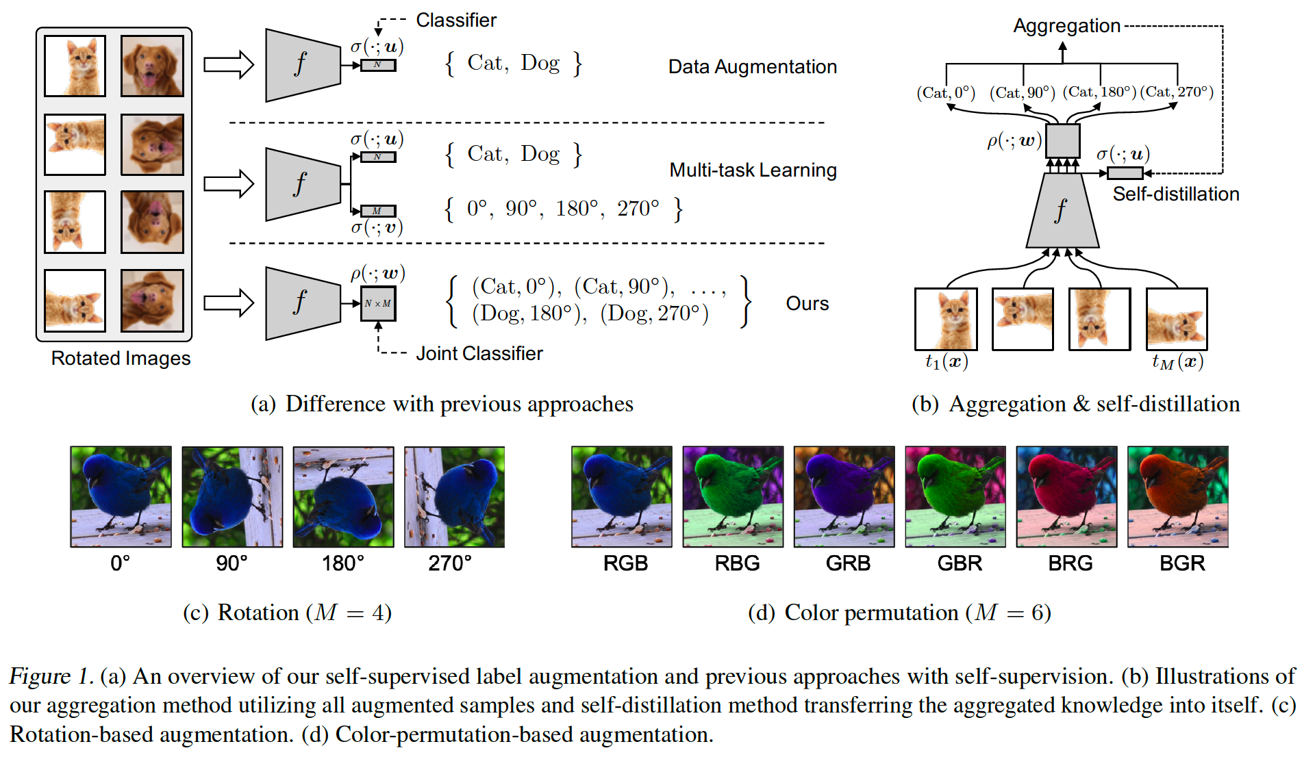
(1) Multi-task Learning with Self-supervision

transformation-based self-supervised learning

• learn to predict which transformation is applied
• usually use 2 losses (multi-task learning)

Loss function :

\(\begin{aligned} &\mathcal{L}_{\mathrm{MT}}(\boldsymbol{x}, y ; \boldsymbol{\theta}, \boldsymbol{u}, \boldsymbol{v}) =\frac{1}{M} \sum_{j=1}^M \mathcal{L}_{\mathrm{CE}}\left(\sigma\left(\tilde{\boldsymbol{z}}_j ; \boldsymbol{u}\right), y\right)+\mathcal{L}_{\mathrm{CE}}\left(\sigma\left(\tilde{\boldsymbol{z}}_j ; \boldsymbol{v}\right), j\right) \end{aligned}\).

• \(\left\{t_j\right\}_{j=1}^M\) : pre-defined transformations
• \(\tilde{\boldsymbol{x}}_j=t_j(\boldsymbol{x})\) : transformed sample by \(t_j\)
• \(\tilde{\boldsymbol{z}}_j=f\left(\tilde{\boldsymbol{x}}_j ; \boldsymbol{\theta}\right)\) : embedding
• \(\sigma(\cdot ; \boldsymbol{u})\) : classifier ( for primary task )
• \(\sigma(\cdot ; \boldsymbol{v})\) : classifier ( for self-supervised task )

\(\rightarrow\) forces the primary classifier to be invariant to transformation

LIMITATION

• depending on the type of transformation….

  \(\rightarrow\) might hurt performance!

• ex) rotation … number 6 & 9

(2) Eliminating Invariance via Joint-label Classifier

• remove the unnecessary INVARIANT propoerty of the classifier \(\sigma(f(\cdot) ; \boldsymbol{u})\)

• instead, use a JOINT softmax classifier \(\rho(\cdot ; \boldsymbol{w})\)

  • joint probability : \(P(i, j \mid \tilde{\boldsymbol{x}})=\rho_{i j}(\tilde{\boldsymbol{z}} ; \boldsymbol{w})=\exp \left(\boldsymbol{w}_{i j}^{\top} \tilde{\boldsymbol{z}}\right) / \sum_{k, l} \exp \left(\boldsymbol{w}_{k l}^{\top} \tilde{\boldsymbol{z}}\right)\)

• Loss function : \(\mathcal{L}_{\mathrm{SLA}}(\boldsymbol{x}, y ; \boldsymbol{\theta}, \boldsymbol{w})=\frac{1}{M} \sum_{j=1}^M \mathcal{L}_{\mathrm{CE}}\left(\rho\left(\tilde{\boldsymbol{z}}_j ; \boldsymbol{w}\right),(y, j)\right)\)

  • \(\mathcal{L}_{\mathrm{CE}}(\rho(\tilde{\boldsymbol{z}} ; \boldsymbol{w}),(i, j))=-\log \rho_{i j}(\tilde{\boldsymbol{z}} ; \boldsymbol{w})\).

• only increases the number of labels

  ( number of additional parameters are very small )

• \(\mathcal{L}_{\mathrm{MT}}\) and \(\mathcal{L}_{\mathrm{SLA}}\) :

• consider the same set of multi-labels

Aggregated Inference

• do not need to consider \(N \times M\) labels

  ( because we already know which transformation is applied )

• make prediction using conditional probability

  • \(P\left(i \mid \tilde{\boldsymbol{x}}_j, j\right)=\exp \left(\boldsymbol{w}_{i j}^{\top} \tilde{\boldsymbol{z}}_j\right) / \sum_k \exp \left(\boldsymbol{w}_{k j}^{\top} \tilde{\boldsymbol{z}}_j\right)\).

• for all possible transformations…

  • aggregate the conditonal probabilities!
  • acts as an ensemble model
  • \(P_{\text {aggregated }}(i \mid \boldsymbol{x})=\frac{\exp \left(s_i\right)}{\sum_{k=1}^N \exp \left(s_k\right)}\).

Self-distillation from aggregation

• requires to compute \(\tilde{\boldsymbol{z}}_j=f\left(\tilde{\boldsymbol{x}}_j\right)\) for all \(j\)

  \(\rightarrow\) \(M\) times higher computation cost than single inference

• Solution : perform self-distillation

  • from ) aggregated knowledge \(P_{\text {aggregated }}(\cdot \mid \boldsymbol{x})\)

  • to ) another classifier \(\sigma(f(\boldsymbol{x} ; \boldsymbol{\theta}) ; \boldsymbol{u})\)

    \(\rightarrow\) can maintain the aggregated knowledge, using only \(\boldsymbol{z}=f(\boldsymbol{x})\)

• objective function :

  \[\begin{aligned} \mathcal{L}_{\mathrm{SLA}+\mathrm{SD}}(\boldsymbol{x}, y ; \boldsymbol{\theta}, \boldsymbol{w}, \boldsymbol{u})=& \mathcal{L}_{\mathrm{SLA}}(\boldsymbol{x}, y ; \boldsymbol{\theta}, \boldsymbol{w}) \\ &+D_{\mathrm{KL}}\left(P_{\text {aggregated }}(\cdot \mid \boldsymbol{x}) \mid \mid \sigma(\boldsymbol{z} ; \boldsymbol{u})\right) \\ &+\beta \mathcal{L}_{\mathrm{CE}}(\sigma(\boldsymbol{z} ; \boldsymbol{u}), y) \end{aligned}\]