Bootstrap Your Own Latent , A New Approach to Self-Supervised Learning

0. Abstract

BYOL ( = Bootstrap Your Own Latent )

new appraoch to self-supervised image representation learning
2 NN
- (1) online NN
- (2) target NN
\(\rightarrow\) interact & learn from each other

Online Network

predict the target network representation of the same image, under different augmentation

Target Network

Previous approaches

“learn representations by predicting different views of same image”
Problem : collapsed representations
- representation that is constant across views is always fully predictive
Solution ( by contrastive methods ) :
- reformulate to discrimination problem
  
  \(\rightarrow\) discriminate between representation of another augmented view
( still problem …. requires comparing each representation of an augmented view with many negative examples )

Goal : prevent collapse!

use a FIXED randomly initialized network to “produce the targets”

( of course, bad result… )

\(\rightarrow\), but, using FIXED network is better than using FIXED representation

Goal : learn a representation \(y_{\theta}\) , which can be used for downstream tasks

2 Networks : ONLINE & TARGET

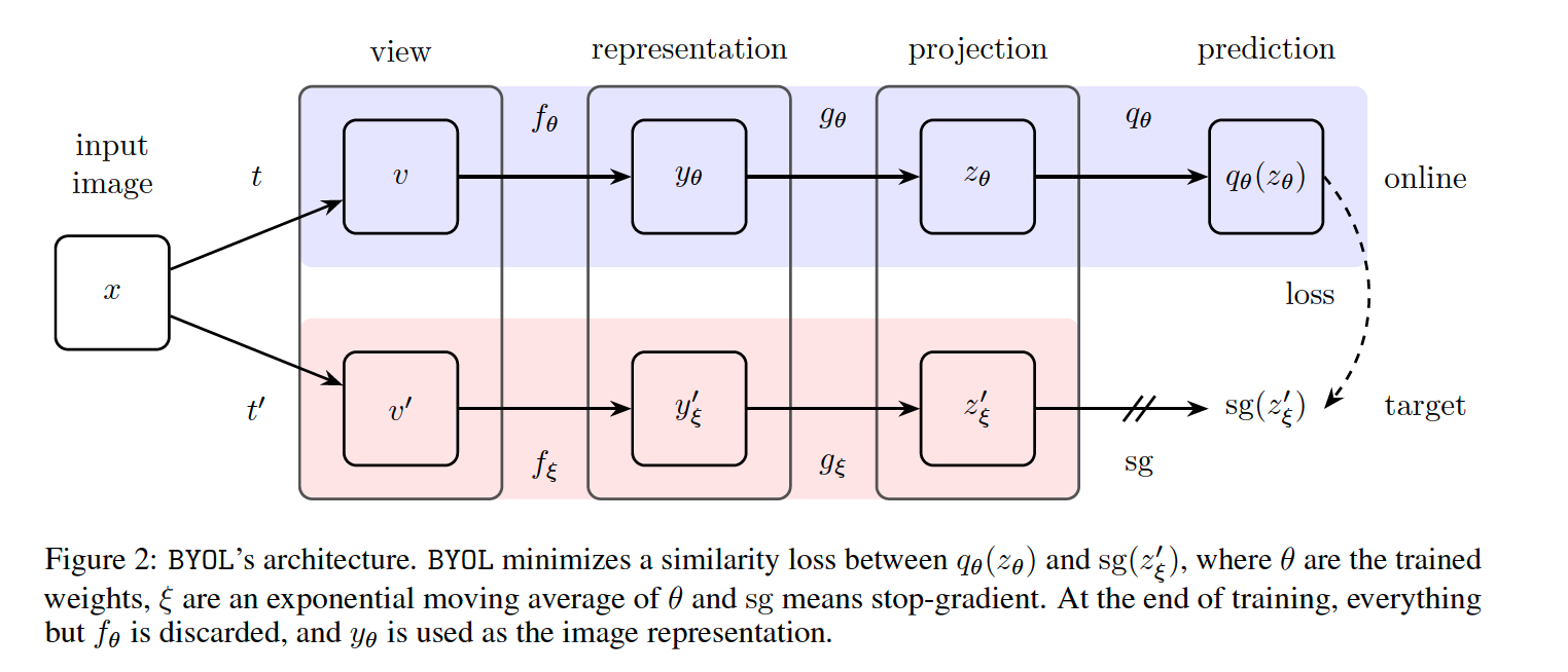
ONLINE network & TARGET network

ONLINE weight : \(\theta\)
TARGET weight : \(\xi\)
3 stages :
- (1) encoder \(f_{\theta}\) & \(f_{\xi}\)
- (2) projector \(g_{\theta}\) & \(g_{\xi}\)
- (3) predictor \(q_{\theta}\) & \(q_{\xi}\)

TARGET network

provides the regression targets for online network
\(\xi\) : exponential moving average of \(\theta\)
target decay rate \(\tau \in[0,1]\)
- \(\xi \leftarrow \tau \xi+(1-\tau) \theta\).

Notation

Image set : \(\mathcal{D}\)
(Uniformly) sampled images : \(x \sim \mathcal{D}\)
2 augmentations : \(\mathcal{T}\) and \(\mathcal{T}^{\prime}\)

\(\rightarrow\) 2 augmented views : \(v \triangleq t(x)\) and \(v^{\prime} \triangleq t^{\prime}(x)\)

Step 1) pass \(v\) into ONLINE network

Step 2) pass \(v^{\prime}\) into TARGET network

output 1 ( = representation ) : \(y_{\xi}^{\prime} \triangleq f_{\xi}\left(v^{\prime}\right)\)
output 2 ( = projection ) : \(z_{\xi}^{\prime} \triangleq g_{\xi}\left(y^{\prime}\right)\)

Step 3) L2 normalization

(1) \(q_{\theta}\left(z_{\theta}\right)\) \(\rightarrow\) \(\overline{q_{\theta}}\left(z_{\theta}\right) \triangleq q_{\theta}\left(z_{\theta}\right) / \mid \mid q_{\theta}\left(z_{\theta}\right) \mid \mid _{2}\)
(2) \(z_{\xi}^{\prime} \triangleq g_{\xi}\left(y^{\prime}\right)\) \(\rightarrow\) \(\bar{z}_{\xi}^{\prime} \triangleq z_{\xi}^{\prime} / \mid \mid z_{\xi}^{\prime} \mid \mid _{2}\)

Step 4) Loss function ( = MSE )

\(\mathcal{L}_{\theta, \xi} \triangleq \mid \mid \overline{q_{\theta}}\left(z_{\theta}\right)-\bar{z}_{\xi}^{\prime} \mid \mid _{2}^{2}=2-2 \cdot \frac{\left\langle q_{\theta}\left(z_{\theta}\right), z_{\xi}^{\prime}\right\rangle}{ \mid \mid q_{\theta}\left(z_{\theta}\right) \mid \mid _{2} \cdot \mid \mid z_{\xi}^{\prime} \mid \mid _{2}}\).

Step 5) Symmetrize Loss ( change \(v\) & \(v^{\prime}\) )

\(\mathcal{L}_{\theta, \xi}^{\text {BYOL }}=\mathcal{L}_{\theta, \xi}+\widetilde{\mathcal{L}}_{\theta, \xi}\).

Step 6) Optimization

update w.r.t \(\theta\) only!! ( not \(\xi\) )
\(\begin{aligned} &\theta \leftarrow \operatorname{optimizer}\left(\theta, \nabla_{\theta} \mathcal{L}_{\theta, \xi}^{\text {BYOL }}, \eta\right), \\ &\xi \leftarrow \tau \xi+(1-\tau) \theta \end{aligned}\).