
BEIT: BERT Pre-Training of Image Transformers
Contents
- Abstract
- Methods
- Image Representation
- Backbone Network : Image Transformer
- Pre-Training BEIT : MIM
0. Abstract
self-supervised vision representation model, BEIT
( = Bidirectional Encoder representation from Image Transformers )
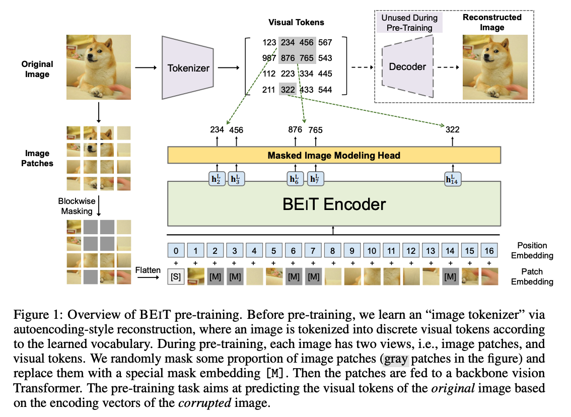
BEIT
- masked image modeling task to pretrain vision Transformers
- each image has two views
- (1) image patches (such as 16×16 pixels)
- (2) visual tokens (i.e., discrete tokens)
Process
- step 1) tokenize the original image into visual tokens
- step 2) randomly mask some image patches
- step 3) feed them to backbone Transformer
Goal :
-
recover the original visual tokens,
based on the corrupted image patches
1. Methods
BEIT
-
encodes input image \(x\) to contextualized vector
-
pretrained by the masked image modeling (MIM) task
( MIM = recover the masked image patches )
-
downstream tasks
- ex) image classification, and semantic segmentation
- append task layers upon pretrained BEIT & fine-tune
(1) Image Representation
2 views of representations
- (1) image patch ( serve as INPUT )
- (2) visual tokens ( serve as OUTPUT )
a) Image Patch
image : split into a sequence of patches
- (from) image \(\boldsymbol{x} \in \mathbb{R}^{H \times W \times C}\)
- (to) \(N=H W / P^2\) patches \(\boldsymbol{x}^p \in \mathbb{R}^{N \times\left(P^2 C\right)}\)
Image patches \(\left\{\boldsymbol{x}_i^p\right\}_{i=1}^N\)
-
step 1) flattened into vectors
-
step 2) linearly projected
( \(\approx\) word embeddings in BERT )
b) Visual Token
represent the image as a sequence of discrete tokens
( = obtained by an “image tokenizer” )
Tokenize …
- (from) image \(\boldsymbol{x} \in \mathbb{R}^{H \times W \times C}\)
- (to) \(\boldsymbol{z}=\left[z_1, \ldots, z_N\right] \in \mathcal{V}^{h \times w}\)
- where the vocabulary \(\mathcal{V}=\{1, \ldots, \mid \mathcal{V} \mid \}\) contains discrete token indices
Image Tokenizer
-
learned by discrete variational autoencoder (dVAE)
-
two modules ( during visual token learning )
-
(1) tokenizer : \(q_\phi(\boldsymbol{z} \mid \boldsymbol{x})\)
-
maps image pixels \(\boldsymbol{x}\) into discrete tokens \(\boldsymbol{z}\)
( according to codebook ( =vocab ) )
-
uniform prior
-
-
(2) decoder : \(p_\psi(\boldsymbol{x} \mid \boldsymbol{z})\)
-
reconstructs the mage \(\boldsymbol{x}\) based on the visual tokens \(\boldsymbol{z}\)
-
Reconstruction objective : \(\mathbb{E}_{\boldsymbol{z} \sim q_\phi(\boldsymbol{z} \mid \boldsymbol{x})}\left[\log p_\psi(\boldsymbol{x} \mid \boldsymbol{z})\right]\)
( discrete? use Gumbel Softmax Trick )
-
-
Details :
- # of visual tokens = # of image patches
- vocab size : \(\mid \mathcal{V} \mid =8192\)
(2) Backbone Network : Image Transformer
( use the standard Transformer as the backbone )
a) Input ( of Transformer ) :
-
sequence of image patches \(\left\{\boldsymbol{x}_i^p\right\}_{i=1}^N\)
( \(N\) = number of patches )
b) Embeddings :
- \(\left\{\boldsymbol{x}_i^p\right\}_{i=1}^N\) are linearly projected to \(\boldsymbol{E} \boldsymbol{x}_i^p\)
- where \(\boldsymbol{E} \in \mathbb{R}^{\left(P^2 C\right) \times D}\)
- add learnable 1d positional embeddings : \(\boldsymbol{E}_{\text {pos }} \in \mathbb{R}^{N \times D}\)
- final output embedding : \(\boldsymbol{H}_0=\left[\boldsymbol{e}_{[\mathrm{S}]}, \boldsymbol{E} \boldsymbol{x}_i^p, \ldots, \boldsymbol{E} \boldsymbol{x}_N^p\right]+\boldsymbol{E}_{\text {pos }}\)
c) Encoder :
-
contains \(L\) layers of Transformer blocks
- \(\boldsymbol{H}^l=\operatorname{Transformer}\left(\boldsymbol{H}^{l-1}\right)\).
-
output vectors of the last layer : \(\boldsymbol{H}^L=\left[\boldsymbol{h}_{[\mathrm{s}]}^L, \boldsymbol{h}_1^L, \ldots, \boldsymbol{h}_N^L\right]\)
( \(\boldsymbol{h}_i^L\) : vector of the \(i\)-th patch )
\(\rightarrow\) encoded representations for the image patches
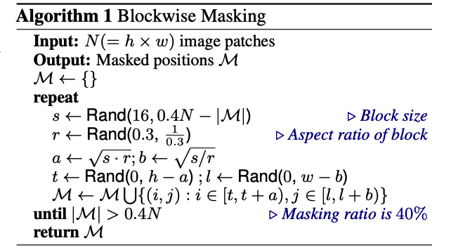
(3) Pre-Training BEIT : MIM
randomly mask some % of image patches
& predict the visual tokens ( corresponding to the masked patches )
Notation
- Input image : \(\boldsymbol{x}\)
- \(N\) image patches : \(\left(\left\{\boldsymbol{x}_i^p\right\}_{i=1}^N\right)\)
- \(N\) visual tokens : \(\left(\left\{z_i\right\}_{i=1}^N\right)\)
- Masked positions : \(\mathcal{M} \in\{1, \ldots, N\}^{0.4 N}\)
- randomly mask approximately \(40 \%\) image patches
Replace the masked patches with a learnable embedding \(e_{[M]} \in \mathbb{R}^D\).
\(\rightarrow\) corrupted image patches : \(x^{\mathcal{M}}=\left\{\boldsymbol{x}_i^p: i \notin \mathcal{M}\right\}_{i=1}^N \bigcup\left\{\boldsymbol{e}_{[M]}: i \in \mathcal{M}\right\}_{i=1}^N\)
\(x^{\mathcal{M}}\) are then fed into the \(L\)-layer Transformer
\(\rightarrow\) final hidden vectors : \(\left\{\boldsymbol{h}_i^L\right\}_{i=1}^N\)
( = regarded as encoded representations of the input patches )
Classification ( with softmax classifier )
- classify for each masked position \(\left\{\boldsymbol{h}_i^L: i \in \mathcal{M}\right\}_{i=1}^N\)
- \(p_{\mathrm{MIM}}\left(z^{\prime} \mid x^{\mathcal{M}}\right)=\operatorname{softmax}_{z^{\prime}}\left(\boldsymbol{W}_c \boldsymbol{h}_i^L+\boldsymbol{b}_c\right)\).
- \(x^{\mathcal{M}}\) : corrupted image
- \(\boldsymbol{W}_c \in \mathbb{R}^{ \mid \mathcal{V} \mid \times D}\) and \(\boldsymbol{b}_c \in \mathbb{R}^{ \mid \mathcal{V} \mid }\)
Pre-training objective
-
maximize the log-likelihood of the correct visual tokens \(z_i\) given the corrupted image:
-
\(\max \sum_{x \in \mathcal{D}} \mathbb{E}_{\mathcal{M}}\left[\sum_{i \in \mathcal{M}} \log p_{\operatorname{MIM}}\left(z_i \mid x^{\mathcal{M}}\right)\right]\).